


Abstract
We report on the development of MPI-AMRVAC version 2.0, which is an open-source framework for parallel, grid-adaptive simulations of hydrodynamic and magnetohydrodynamic (MHD) astrophysical applications. The framework now supports radial grid stretching in combination with adaptive mesh refinement (AMR). The advantages of this combined approach are demonstrated with one-dimensional, two-dimensional, and three-dimensional examples of spherically symmetric Bondi accretion, steady planar Bondi–Hoyle–Lyttleton flows, and wind accretion in supergiant X-ray binaries. Another improvement is support for the generic splitting of any background magnetic field. We present several tests relevant for solar physics applications to demonstrate the advantages of field splitting on accuracy and robustness in extremely low-plasma β environments: a static magnetic flux rope, a magnetic null-point, and magnetic reconnection in a current sheet with either uniform or anomalous resistivity. Our implementation for treating anisotropic thermal conduction in multi-dimensional MHD applications is also described, which generalizes the original slope-limited symmetric scheme from two to three dimensions. We perform ring diffusion tests that demonstrate its accuracy and robustness, and show that it prevents the unphysical thermal flux present in traditional schemes. The improved parallel scaling of the code is demonstrated with three-dimensional AMR simulations of solar coronal rain, which show satisfactory strong scaling up to 2000 cores. Other framework improvements are also reported: the modernization and reorganization into a library, the handling of automatic regression tests, the use of inline/online Doxygen documentation, and a new future-proof data format for input/output.
Export citation and abstract BibTeX RIS
1. Introduction
The solar and astrophysical research community can benefit from a whole array of publicly available software frameworks that are suited to modeling instrinsically multi-scale problems on modern computing infrastructure. A recurring ingredient in coping with the multi-scale nature is their capability of using adaptive mesh refinement (AMR). This is essential, e.g., in coping with Sun-to-Earth modeling of solar coronal mass ejections (Manchester et al. 2004), in many applications which extend magnetohydrodynamics (MHD) into special relativistic regimes (Keppens et al. 2012; Mignone et al. 2012), in applications recreating conditions in laser–plasma interactions (Tzeferacos et al. 2015), in simulations focusing on the formation and early evolution of disk galaxies in magnetized interstellar medium (Wang & Abel 2009), or in fact in many problems where self-gravitational collapse is at play and AMR-MHD is combined with Poisson solvers (Ziegler 2005a). AMR-MHD is currently available in a large—and still growing—variety of codes, e.g., BATS-R-US (Powell et al. 1999), FLASH (Fryxell et al. 2000; Lee & Deane 2009), RIEMANN (Balsara 2001), MPI-AMRVAC (Keppens et al. 2003, 2012), NIRVANA (Ziegler 2005b), RAMSES (Fromang et al. 2006), PLUTO (Mignone et al. 2007), ATHENA (Stone et al. 2008), AstroBEAR (Cunningham et al. 2009), ..., and it drove the development of novel MHD algorithms (e.g., Rossmanith 2004; Fromang et al. 2006; Stone et al. 2008; Cunningham et al. 2009). For example, recent Sun-to-Earth model efforts combine the use of a near-Sun overset yin–yang grid, with a cartesian AMR grid to handle the further heliosphere dynamics (Feng et al. 2011), where the AMR part is based on the PARAMESH (MacNeice et al. 2000) implementation.
In this paper, we report an upgrade to the open source MPI-AMRVAC software (Porth et al. 2014c), which was initially developed as a tool to study hyperbolic partial differential equation (PDE) systems such as the Euler system or ideal MHD with patch-based or hybrid-block-based AMR meshes (Keppens et al. 2003; van der Holst & Keppens 2007). Using the loop annotation syntax (LASY) (Tóth 1997), the software is written in Fortran 90 plus Perl annotations so that the same code can be translated by a Perl preprocessor into any dimensional pure Fortran code before compilation. With the LASY implementation, typical expressions appearing in multidimensional simulation codes can be written in a much more concise form, less prone to mistakes. Adding geometric source terms, one-to-three-dimensional AMR meshes can be in Cartesian, polar, cylindrical, or spherical coordinate systems. As a result, MPI-AMRVAC matured to a multi-physics software framework with modules to handle special relativistic hydro to MHD problems (Meliani et al. 2007; van der Holst et al. 2008; Keppens et al. 2012) and with the ability to couple different PDE models in localized domain regions across block-based AMR meshes (Keppens & Porth 2014). To ensure efficient scaling on realistic applications, the AMR strategy evolved to a pure quadtree-octree block-based AMR hierarchy (Keppens et al. 2012; Porth et al. 2014c). In Porth et al. (2014c), we reported on conservative fourth-order finite difference schemes, and new modules to allow simulating hydrodynamics with dust coupling (Hendrix & Keppens 2014) or Hall MHD (Leroy & Keppens 2017). Selected applications of MPI-AMRVAC focus on shock-dominated special relativistic hydro problems in the context of gamma-ray burst blast waves and their afterglow (Meliani & Keppens 2010; Vlasis et al. 2011), and up to full three-dimensional (3D) modeling of the precessing jets in the X-ray binary SS433 (Monceau-Baroux et al. 2014). Relativistic MHD applications studied propagation aspects of magnetized relativistic jets (Keppens et al. 2008), to detailed modeling of the Crab Nebula (Porth et al. 2014a, 2014b). Newtonian hydro applications addressed accretion processes onto compact objects (El Mellah & Casse 2015), the wind collision and dust redistribution in the Wolf-Rayet 98a rotating pinwheel nebula (Hendrix et al. 2016), and MHD is employed in many solar challenges, such as modeling the in situ formation of solar prominences (Xia et al. 2012, 2014; Xia & Keppens 2016), solar coronal rain dynamics (Fang et al. 2013, 2015; Xia et al. 2017), or the initiation of coronal mass ejections (Mei et al. 2017; Zhao et al. 2017).
Recently, general relativistic fluid or plasma dynamics in arbitrary spacetimes can be handled by the black hole accretion code (BHAC), an MPI-AMRVAC spin-off that shares its algorithmic versatility and efficient block-based AMR ability (Porth et al. 2017). MPI-AMRVAC development focused on more Newtonian physics, with solar physics oriented functionality to extrapolate vector magnetic field distributions into coronal volumes using magnetofrictional methods (Guo et al. 2016b, 2016c). This augments the earlier potential to linear-force-free field extrapolation in local Cartesian boxes or global spherical coordinates (Porth et al. 2014c), and paves the way to future data-driven solar applications. Driven by these ambitions as well as by several recent applications, many new functionalities have been developed. Since several of them can be of general interest to the astrophysical community and have not been documented elsewhere, we present them here in more detail, with an emphasis on demonstrating their advantages in a series of tests. We start with hydro to MHD applications where we employ radially stretched meshes in curvilinear coordinates in Section 2. This is shown to be crucial in accretion flow (or outflow) setups, where we wish to concentrate resolution around the accreting object near the inner radial boundary and prevent deformation of the cells at large radial distances, preserving cell shape for the consistent resolution and accuracy. For MHD problems, the technique of magnetic field splitting, invented to handle low-β shock-dominated plasma, was originally limited to potential (current-free) background fields (Tanaka 1994). We report an extension of this technique to allow the time-independent split-off part to be any magnetic field in Section 3. To accurately solve anisotropic thermal conduction in magnetized plasma, we present an extension to 3D of a slope-limited symmetric scheme in Section 4, which is shown to handle sharp temperature gradients very well. We report on scaling tests where these methods are adopted in full 3D coronal rain applications in Section 5. Other useful, more generic code framework improvements are reported in Section 6, and collectively define what we introduce as MPI-AMRVAC 2.0.
2. Radially Stretched Meshes
Modeling of many physical problems relies on the use of spherical, polar, or cylindrical meshes, and on resolving the evolution of gas or plasma flows over several spatial orders of magnitude. In astrophysical configurations, the interplay between gravitation and in- or outflows is a recurring ingredient that would benefit from combining, e.g., a spherical mesh with a gradual radial stretching of the cells, in combination with block-adaptivity. Here, we report on one-dimensional (1D) to fully 3D tests or applications where this is exploited.
2.1. 1D Bondi Transonic Accretion
The simplest hydrodynamical representation of the accretion of matter by a point mass was analyzed early on by Bondi (1952). It is an isotropic problem where only radial dependencies and components are considered. It describes how a non-zero temperature flow moving at a subsonic speed at infinity toward a central object of mass M* can establish a steady, smooth, and transonic inflow solution. This unique continuous, transonic inflow solution vr(r) does not display any shock. Provided the evolution is adiabatic, it means that the flow is isentropic: the pressure p(r) can be deduced from the mass density  , using the fixed adiabatic index γ of the flow (
 is independent of radius r). To illustrate how we make the equations dimensionless, let us look at the physical equation of conservation of the linear momentum:

where all quantities are in physical units, M* is the mass of the accretor and G is the gravitational constant. We now adopt the following normalization quantities:
- 1.the mass density at infinity,
 ,
, - 2.the sound speed at infinity, c∞,
- 3.the radius.


Using these scalings, the mass per unit time crossing a sphere of a given radius (the mass accretion rate,  ), the pressure, and the time are normalized with
  ,
,  , and
, and  respectively. In the equation above, if we replace ρ, vr, p, r, and t with the product of a dimensionless number by the associated normalization quantity stated above (for instance ρ becomes
  ), we obtain :

which leads to the fully dimensionless equation (4) below. From now on, we omit the tildes and work exclusively with normalized dimensionless variables. Finally, notice that the analytic expressions below assume the specific case of a zero speed at infinity, but the conclusions below remain qualitatively the same in the general case.
The fundamental equations of this problem are the mass continuity equation

linear momentum conservation with gravity as a source term

and the isentropic relation between (scaled) pressure and density as  . The steady-state solution admits a radius at which it becomes supersonic, called the sonic radius rs, whose expression can be analytically derived to be
  . The isothermal case (i.e.,
  ) has its associated sonic radius at
  (this is identical for the corresponding unique outflowing Parker isothermal wind solution). The normalized mass accretion rate can also be determined from the adiabatic index:

For derivations of the above results, in the more general case of a non-zero subsonic speed at infinity, the reader might refer to Section 4.2 of El Mellah (2016). Below r = 1 (i.e., below the position of the scaling radius R0) the properties of the flow significantly depart from their values at infinity. For an adiabatic index close to the maximum value of 5/3 that it can take, the sonic radius rs becomes very small. We want to have the sonic radius within the simulation space, to have a trivial inner boundary treatment where inflow is supersonic. It then becomes advantagous to resort to a stretched mesh.
We work on domains extending from a radius of 0.01 (inner boundary) to 10 (outer boundary). We rely on a second-order two-step Harten–Lax–van Leer–Contact (HLLC) method (Toro et al. 1994), both for the predictor and the full time step, with the Koren slope limiter (Vreugdenhil & Koren 1993) used in the limited reconstruction of the primitive variables ρ and vr, to obtain cell-face values. To design our initial conditions and fix the outer r = 10 inflow boundary conditions, we reformulate the fundamental equations to obtain a transcendental equation which indirectly gives the mass density as a function of radius r:

We numerically solve this relation with a Newton–Raphson method, which behaves correctly except very near the sonic radius where the algorithm may yield non-monotonous results. In this restricted region, we compute the mass density profile by linearly interpolating between points further away from the sonic radius. The obtained mass density profile is used as the initial condition and sets the fixed mass density in the ghost cells beyond r = 10. For the linear momentum  , we deduce its radial profile from Equation (5) and similarly implement it both as initial condition and as forced outer boundary condition. For the inner boundary conditions, we copy the mass density in the ghost cells and then guarantee the continuity of the mass flux and Bernoulli invariant (as in El Mellah & Casse 2015). We then use MPI-AMRVAC to time-advance the solution to retrieve the stationary analytical solution, on three different kinds of radial spherical meshes :
- 1.a non-stretched grid with a total number of cells N = 16388, without AMR,
- 2.a stretched grid with a much reduced total number of cells (N = 132), stretched such that the relative resolution at the inner boundary remains the same as for the previous grid, without AMR,
- 3.the same stretched grid as above, but with a total of five levels of mesh refinement, where blocks which contain the analytic sonic radius are refined. The refined grid is computed at the initial state and does not evolve thereafter (static AMR).
Within a few dynamical times, the profiles relax toward a numerical equilibrium close to the solution determined with the Newton–Raphson above. To quantify the relaxed steady states, we measure the position of the sonic radius obtained for each of the three meshes, and this for four different adiabatic indexes. The results are summarized in Figure 1. By eye, it is impossible to distinguish the numerically obtained sonic radii (dots) from the analytic solution (dashed curve) displayed in the upper panel, whatever the mesh. Therefore, we plotted the relative differences in the three lower panels for the non-stretched grid (b), a stretched grid (c), and a stretched grid with AMR (d). The error bars are evaluated by considering one hundredth of the spatial resolution in the vicinity of the sonic radius. We can conclude from those results that analytic sanity checks such as the position of the sonic radius are retrieved within a few tenths of percent with MPI-AMRVAC.

Figure 1. (a) Sonic radius rs relative to its value  at
at  as a function of the adiabatic index. The dashed line represents the analytic solution given by
  , while the four dots are the sonic radii measured from the steady-state solution computed by MPI-AMRVAC. (b)–(d) Relative differences between the analytic and computed sonic radii for a non-stretched high-resolution grid, a stretched grid, and a stretched grid with AMR. The errorbars are represented in red and computed as explained in the text.
Download figure:
Standard image High-resolution imageApart from this local agreement on the sonic point location, we can also quantify an error estimate for the entire relaxed mass density profiles obtained. For the case where  , we compare runs with different AMR levels employing stretched meshes, to the relaxed mass density profile obtained with the non-stretched, high-resolution mesh above. We compute the L2-norm between data points on stretched, AMR meshes and their counterpart on the non-stretched mesh (linearly interpolated to the same radial positions). Figure 2 shows that the matching between the solutions obtained increases as the number of maximum AMR levels rises.

Figure 2. Quantification of the departure of the relaxed mass density profiles obtained with stretched meshes, for different AMR levels, with respect to the profile obtained with a non-stretched mesh. Those results were obtained for  .
.
Download figure:
Standard image High-resolution image2.2. Radial Stretching Principle
Radial stretching is introduced both to decrease the number of radial cells and, in two-dimensions (2D) and 3D, to prevent the deformation of cells when the radius of the inner radial boundary of the grid is orders of magnitude smaller than the radius of the outer boundary. To keep a constant cell aspect ratio all over a 2D  grid, the radial step size
  must obey the following relation :

where ri is the local radius,  the uniform angular step (the latitudinal one for a spherical
  mesh where θ is the colatitude) and ζ is a fixed aspect ratio. Since the radial step is then proportional to the radius, we obtain a kind of self-similar grid from the innermost to the outermost regions. We set the radial position ri of the center of any cell indexed i mid-way between the two surrounding interfaces,
  and
and  , see Figure 3. The recursive relationship which builds up the sequence of radial positions for the cell centers is given by

where  is the radial step of cell i. Inserting equation (7) yields :

Hereafter, q is called the scaling factor. We fix the radii of the inner and outer radial boundaries of the domain, rin and rout respectively, along with the total number of cells in the radial direction N (excluding the ghost cells). The scaling factor is then computed from equation (9) applied to the two boundaries:  . We can derive the required aspect ratio for a radially stretched grid:

For a stretching smooth enough and a usual number (typically two) of ghost cells, the radial positions of the inner ghost cells remain positive.

Figure 3. Uni-dimensional representation of the radial stretching with the cell centers marked with a vertical line and the cell edges with a back-to-back double bracket. The cell centers are always mid-way between two consecutive edges, but the reverse is not true. The inner and outer edges are marked by longer vertical lines with dashes. There are two ghost cells on each side (n = 2) in this example.
Download figure:
Standard image High-resolution imageAs should be clear from our example applications, the stretched grid is created accordingly to the type of symmetry (cylindrical or spherical) and to the dimensionality (1D, 2D, or 3D). The numerical schemes incorporate the variable radial step size where needed. The coupling between stretched grids and block-based AMR has been made possible by computing a scaling factor for each AMR level. Since children blocks at the next level span the same radial range as the mother block but with twice as many cells, the scaling factor  of the children blocks at level
  can be obtained from the scaling factor ql of the mother block at level l via
  .
.
The time gain can be estimated by writing the ratio of the number of radial cells in a non-stretched versus a stretched grid, with the same absolute radial step at the inner boundary. It approximately amounts to:

which quickly rises when  exceeds a few tens. Moreover, in combination with AMR, the stretched grid enables us to resolve off-centered features (see, e.g., our 3D application in Section 2.4), without lowering the time step, if the latter is dominated by dynamics within the innermost regions. In the previous section on 1D Bondi accretion, the number of cells for an accurate solution could be reduced by two orders of magnitude.
2.3. The 2.5D Bondi–Hoyle–Lyttleton Problem
A truly 2D accretion-type problem is the Bondi–Hoyle–Lyttleton (BHL) model designed by Hoyle & Lyttleton (1939) and Bondi & Hoyle (1944) (for a more detailed review of the BHL model and its refinements, see Edgar 2004; El Mellah 2016). The major change with respect to the 1D Bondi flow is that there is now a supersonic bulk planar motion of the flow with respect to the accretor, at speed  , which has two serious consequences:
- 1.the geometry of the problem is no longer isotropic but is still axisymmetric (around the axis through the accretor and with direction set by the speed of the inflow at infinity),
- 2.since the flow is supersonic at infinity, there can be a bow shock induced by the interaction with the accretor. The isentropic assumption we used to bypass the energy equation in Section 2.1 no longer holds.
Analytic considerations point to a formation of the shock at a spatial scale of the order of the accretion radius  . This radius is close to the size of the accretor, when we study stars accreting the wind of their companion in binary systems (Chen et al. 2017). However, for compact accretors which have an associated Schwarzschild radius
  , the contrast between accretor size and the scale at which the flow is deflected by the gravitational influence of the accretor becomes important, since

where c is the speed of light. For realistic speeds  of stellar winds in wind-dominated X-ray binaries for instance, it means that the accretor is 4 to 5 orders of magnitude smaller than the shock forming around it. To bridge the gap between those scales, a stretched grid is mandatory.
This has been done with MPI-AMRVAC in El Mellah & Casse (2015), where we solved the hydro equations on a 2D  grid combined with axisymmetry about the ignored φ direction. The set of equations to solve now include the energy equation, also with work done by gravity appearing as a source term, where the energy variable
  is used to deduce the pressure. In the simulations, we work with an adiabatic index representative of a monoatomic gas,
  . The equations solved write as:


The terms on the RHS are handled in geometric and gravitational source terms.
Fortunately, not all quantities require an inner rin boundary which matches the physical size of the accretor. For instance, Ruffert (1994) quantified the impact of the size of the inner boundary rin on the measured mass accretion rates at the inner boundary,  (see Figure 5.3 in El Mellah 2016). The result is that
  matches the analytic value provided one reaches the sonic radius. But, as explained in the previous 1D Bondi test, and as can be seen in Figure 1, the sonic radius drops to zero for
  . Ruffert (1994) showed that to retrieve the analytic value of the mass accretion rate within a few percent, rin must be below a hundredth of the accretion radius. Therefore, in the simulations where
  , we need to span at least 3 orders of magnitude: while the outer boundary lies at 8Racc, the inner boundary has a radius of a thousand times the accretion radius. With a resolution of 176 × 64 cells in the
  plane (without the ghost cells), it gives an aspect ratio of 1.04 (and a scaling factor of 1.05).
The steady solution has the supersonic planar outflow upstream, suddenly transitioning to a subsonic inflow at the bow shock. Then, part of this now subsonic inflow is still accreted in a continuous Bondi-type transonic fashion in the wake of the accretor. Solutions for different Mach numbers  of the supersonic planar inflow are compared in Figure 4, showing density variations in a zoomed-in fashion. The upstream conditions at 8Racc are set by the ballistic solutions (Bisnovatyi-Kogan et al. 1979) and the downstream boundary condition is continuous (with a supersonic outflow). At the inner boundary, we enforce the same boundary conditions as described in Section 2.1, with a continuous
  . MPI-AMRVAC provides a steady solution on a stretched (non-AMR) grid which matches the orders of magnitude mentioned above: the position of the detached bow shock, the jump conditions at the shock, as well as the inner mass accretion rate (El Mellah & Casse 2015). In particular, we retrieve a topological property derived by Foglizzo & Ruffert (1996) concerning the sonic surface, deeply embedded in the flow and anchored into the inner boundary, whatever its size (see the solid black contour denoting its location in the zoomed views in Figure 4).

Figure 4. Logarithmic color maps of the density for Mach numbers at infinity of 8 (left panels) and 2 (right panels). Some streamlines have been represented (solid white) and the two dotted black contours stand for the Mach-1 surface. Zoomed-in views of the central area by a factor of 20 (center) and 400 (right).
Download figure:
Standard image High-resolution image2.4. 3D Clumpy wind Accretion in Supergiant X-Ray Binaries
A third hydrodynamic application of radially stretched AMR grids generalizes the 2D (spherical axisymmetric) setup above to a full 3D case. In a forthcoming paper (I. El Mellah et al. 2018, in preparation), we use a full 3D spherical mesh to study wind-accretion in supergiant X-ray binaries, where a compact object orbits an evolved mass-losing star. In these systems, the same challenge of scales identified by Equation (12) is at play, and the BHL shock-dominated, transonic flow configuration is applicable. In realistic conditions, the wind of the evolved donor star is radiatively driven and clumpy, making the problem fully time-dependent. We model the accretion process of these clumps onto the compact object, where the inhomogeneities (clumps) in the stellar wind enter a spherically stretched mesh centered on the accreting compact object, and the clump impact on the time-variability of the mass accretion rate is studied. The physics details will be provided in that paper; here we emphasize how the 3D stretched AMR mesh is tailored to the problem at hand. The initial and boundary conditions are actually derived from the 2.5D solutions described above, while a seperate 2D simulation of the clump formation and propagation in the companion stellar wind serves to inject time-dependent clump features in the supersonic inflow.
The use of a 3D spherical mesh combined with explicit time stepping brings in additional challenges since the time step  must respect the Courant–Friedrich–Lewy (CFL) condition. Since the azimuthal line element is
  with colatitude θ, it means that the time step obeys

The axisymmetry adopted in the previous section avoided this complication. As a consequence, the additional cost in terms of number of iterations to run a 3D version of the setup presented in the previous section is approximately

where  is the colatitude of the first cell center just off the polar axis. For a resolution on the base AMR level of 64 cells spanning
  to
to  , it means a time step 40 times smaller compared to the 2D counterpart. Together with the additional cells in the azimuthal direction, this makes a 3D setup much more computationally demanding.
We compromise on this aspect by using an AMR mesh which deliberately exploits a lower resolution at the poles, while still resolving all relevant wind structures. Since the clumps embedded in the supersonic inflow are small-scale structures, we need to enable AMR (up to four levels in the example of Figure 5) in the upstream hemisphere to resolve them, in particular at the outer edge of the mesh where the radially stretched cells have the largest absolute size on the first AMR level. At the same time, we are only interested in the fraction of the flow susceptible to be accreted by the compact object, so we can inhibit AMR refinement in the downstream hemisphere, except in the immediate vicinity of the accretor (below the stagnation point in the wake). We also prevent excessive refinement in the vicinity of the accretor (no refinement beyond the third level in Figure 5) since the stretching already provides more refined cells. Finally, in the upstream hemisphere, we favor AMR refinement in the accretion cylinder, around the axis determined by the direction of the inflow velocity. Note that this axis was the symmetry polar axis in the previous 2.5D setup in Section 2.3, but this is different in the present 3D setup, where the polar axis is above and below the central accretor. In the application to study supergiant X-ray binary accretion, together with geometrically enforced AMR, we use dynamic AMR with a refinement criterion on the mass density to follow the flow as it is accreted onto the compact object.

Figure 5. Two slices of the upper hemisphere of a spherical mesh with four levels of refinement, as used in a study of time-dependent wind-accretion onto a compact object. User-defined restrictions on AMR prevent the grid to be refined in some areas (e.g., in the downstream hemisphere, where the y-coordinate is negative) far from the inner boundary and in the vicinity of the polar z-axis). We further restrict the maximum level of refinement to three in the vicinity of the inner boundary and allow for maximum refinement in the outer regions of the upstream hemisphere close to the y-axis. This corresponds to the supersonic inflow area where clumps enter the grid.
Download figure:
Standard image High-resolution image2.5. Trans-Alfvénic Solar Wind
To simulate the propagation of the solar wind between the Sun and the orbit of the Earth (at 215  ), the use of a spherical stretched grid can also be very important. First, it considerably reduces the amount of cells needed in the simulations (by a factor of 46). Second, it allows us to maintain the same aspect ratio for all the cells in the simulation. We present here the results of 2.5D MHD simulations of the meridional plane of the solar wind, i.e., axisymmetric simulations on a 2D mesh where the three vector components are considered for the plasma velocity and for the magnetic field. This simulation setup also allows us to test the magnetic field splitting (MFS) method discussed in Section 3. Instead of solving the induction equation for the total magnetic field (
 ), one can solve it for the difference with the internal dipole field of the Sun (
 ), where
  represents the dipole field. We will here compare the results of these two setups. In our simulations, the solar wind is generated through the inner boundary (at r = 1
  ), in a fashion similar to Jacobs et al. (2005) and Chané et al. (2005, 2008): the temperature is fixed to
  K, and the number density to
  cm−3, where the azimuthal velocity is set to
  km s−1 to enforce the solar differential rotation of the Sun (θ is the colatitude), and where the radial component of the magnetic field is fixed to the internal dipole value (with Br = 1.1 G at the equator). In addition, close to the equator (at latitudes lower than
  ), in the streamer region, a dead zone is enforced at the boundary by fixing the radial and the latitudinal velocities to zero. The equations solved are the ideal MHD equations plus two source terms: one for the heating of the corona and one for the gravity of the Sun. The heating of the corona is treated as an empirical source term in the energy equation. We follow the procedure described in Groth et al. (2000) with a heating term dependent on the latitude (with a stronger heating at high latitudes) and on the radial distance (the heating decreases exponentially). The inclusion of this source term results in a slow solar wind close to the equatorial plane and a fast solar wind at higher latitudes (see Figure 6).

Figure 6. Axisymmetric 2.5D MHD simulations of the solar wind. The top panels show the color-coded density, the velocity vectors (in white), the magnetic field lines (in black), as well as the Alfvén surface (white line) for two simulations: one where the magnetic field splitting (MFS) method is used (right panel) and one where it is not (left panel). The lower panels show the solar wind characteristics at 1 au: the plasma number density (left panel), radial velocity (middle panel), and the magnetic field magnitude (right panel) for both simulations (with MFS in red and without MFS in blue).
Download figure:
Standard image High-resolution imageThe simulations are performed on a spherical stretch mesh between 1  and 216
  with 380 cells in the radial direction and 224 cells in the latitudinal direction. For these simulations, we do not take advantage of the AMR capabilities of the code and a single mesh level is used (no refinement). The smallest cells (close to the Sun) are 0.014
  , while the largest cells (at 1 au) are 3
  . The equations are solved with a finite-volume scheme, using the two-step HLL solver (Harten et al. 1983) with Koren slope limiters. Powell's method (Powell et al. 1999) is used for the divergence cleaning of the magnetic field. The adiabatic index γ is set to 5/3 in these simulations.
The results of the simulations are shown in Figure 6. The top panels display the plasma density, the velocity vectors, the magnetic field lines, and the Alfvén surface. One can see that both panels are very similar with: (1) a fast solar wind at high latitudes and a slow denser wind close to the equatorial plane, (2) a dense helmet streamer (the reddish region close to the equatorial plane) close to the Sun where the plasma velocity is almost zero, and (3) an Alfvén surface located between 4 and 7.5  in both cases. To highlight the differences between the two simulations, 1D cuts at 1 au are provided in the lower panels of Figure 6 for both simulations. The density profiles are very similar, but the density is marginaly lower when the MFS method is used. For both simulations, the solar wind is, as expected, denser close to the equatorial plane and displays densities in agreement with the average measured density at 1 au. The radial velocity profiles (shown in the middle panel) are nearly identical almost everywhere in both simulations, with a fast solar wind (a bit less than 800 km s−1) at high latitudes, and a slow solar wind (a bit less than 400 km s−1) close to the equator. The only region where the radial velocity profiles marginally differ is on the equatorial plane, where the radial velocity is 4% higher when the MFS method is used. These results are very similar to in situ measurements at 1 au (see, for instance, Phillips et al. 1995). Although the differences are more pronounced for the magnetic field magnitude (right panel), they never exceed 10%. In general, the differences between the two simulations are negligible.
3. Magnetic Field Splitting
When numerically solving for dynamics in solar or planetary atmospheres, the strong magnetic field and its gradients often cause serious difficulties if the total magnetic field is solved for as a dependent variable. This is especially true when both high- and low-β regions need to be computed accurately in shock-dominated interactions. An elegant solution to this problem (Tanaka 1994) is to split the magnetic field  , into a dominating background field
  and a deviation
  , and solve a set of modified equations directly quantifying the evolution of
  . Splitting off this background magnetic field component and only evolving the perturbed magnetic field is more accurate and robust, in the sense that it diminishes the artificial triggering of negative gas pressure in extremely low-β plasma. This background field
  was originally limited to be a time-independent potential field (Tanaka 1994) (as used in the previous section for the solar wind simulation on a stretched mesh), and in this form has more recently led to modifying the formulations of HLLC (Guo 2015) or HLLD (Guo et al. 2016a) MHD solvers, which rely on a 4- to 6-state simplification of the local Riemann fans, respectively. The splitting can also be used for handling background time-dependent, potential fields (Tóth et al. 2008), even allowing for extensions to Hall-MHD physics where challenges due to the dispersive whistler wave dynamics enter. The governing equations for a more general splitting, as revisited below, were also presented in Gombosi et al. (2002), giving extensions to semi-relativistic MHD where the Alfvén speed can be relativistic. The more general splitting form also appears in Feng et al. (2011), although they further apply it exclusively with time-independent, potential fields.
3.1. Governing Equations, Up to Resistive MHD
Here, we demonstrate this MFS method in applications that allow any kind of time-independent magnetic field as the background component, no longer restricted to potential (current-free) settings. At the same time, we wish to also allow for resistive MHD applications that are aided by this more general MFS technique. The derivation of the governing equations employing an arbitrary split in a time-independent  are repeated below, to extend them further on to resistive MHD. The ideal MHD equations in conservative form are given by


where ρ,  ,
,  , and
, and  are the plasma density, velocity, magnetic field, and unit tensor, respectively. In solar applications, gas pressure is
  , assuming full ionization and a solar hydrogen to helium abundance
  , where
  (or the mean molecular weight
  ), while
  is the total energy. Consider
  , where
  is a time-independent magnetic field, satisfying
  and
and  . Equation (20) can be written as

Defining  , then
  and Equation (21) can be written as

When we take the scalar product of Equation (22) with a time-independent  , we can use vector manipulations on the RHS of
  to obtain

Inserting Equation (25) into Equation (24), we arrive at

Therefore, in the ideal MHD system with MFS, we see how a source term appears in the RHS for the momentum Equation (23) that quantifies (partly) the Lorentz force  , where
  , while the energy Equation (26) for E1 features a RHS written as
  for the electric field
  . The induction equation, for a time-invariant
  just writes as before:

For force-free magnetic fields,  , where α is constant along one magnetic field line, we have
  and
and  .
.
For resistive MHD, extra source terms  and
and  , are added on the RHS of the energy Equation (21) and the induction Equation (22), respectively, where
  . Then the energy equation must account for Ohmic heating and magnetic field diffusion, to be written as

The induction equation, extended with resistivity, now gives

Insert Equation (29) to Equation (28), and we have the resistive MHD energy equation in the MFS representation

The induction equation, as implemented, is then written as

In the implementation of the MFS form of the MHD equations, we take the following strategies. Each time when creating a new block, a special user subroutine is called to calculate  at cell centers and cell interfaces which is stored in an allocated array, and then
  is evaluated and stored at cell centers either numerically or analytically with an optional user subroutine. Note that when the block is deleted from the AMR mesh, these stored values are also lost. The third term on the LHS of the momentum Equation (23), energy Equation (26) or (28), and in the induction Equation (27) or (31) is added in the flux computation for the corresponding variable, based on pre-determined
  magnetic field values at the cell interfaces where fluxes are evaluated. The terms on the RHS of all equations are treated as unsplit source terms, which are added in each sub-step of a time integration scheme. We use simple central differencing to evaluate spatial derivatives at cell centers. For example, to compute
  in the physical region of a block excluding ghost cells, we first compute
  in a block region including the first layer of ghost cells, which needs
  at the second layer of ghost cells.
3.2. MFS Applications and Test Problems
We present three tests and one application to demonstrate the validity and advantage of the MFS technique. All three tests are solved with a finite-volume scheme setup combining the HLL solver (Harten et al. 1983) with Čada's compact third-order limiter (Čada & Torrilhon 2009) for reconstruction, and a three-step Runge–Kutta time integration in a dimensionally unsplit approach. We use a diffusive term in the induction equation to keep the divergence of magnetic field under control (Keppens et al. 2003; van der Holst & Keppens 2007; Xia et al. 2014). We adopt a constant index of  . Unless stated explicitly, we employ dimensionless (code) units everywhere, also making
  .
.
3.2.1. 3D Force-free Magnetic Flux Rope
This is a test initialized with a static plasma threaded by a force-free, straight helical magnetic flux rope on a Cartesian grid (see Figure 7). The initial density and gas pressure are uniformly set to unity. The simulation box has a size of 6 × 6 × 6 and is resolved by a  uniform mesh which is decomposed into blocks of
  cells. The magnetic field is non-potential and nonlinearly force-free, as proposed by Low (1977), and is formulated as


We choose free parameters  and k = 0.5 to make the axis of the flux rope align with the x-axis and set Ba = 10. The electric current of this flux rope is analytically found to be

The plasma β ranges from 0.006 to 0.027. The Alfvén crossing time along y-axis across the box is 0.377, determined by the averaged Alfvén speed along the y-axis. This analytical force-free static equilibrium should remain static forever. However, due to the finite numerical diffusion of the numerical scheme adopted, the current in the flux rope slowly dissipates when we do not employ the MFS strategy, thereby converting magnetic energy to internal energy and resulting in (small but) non-zero velocities. After 5 (dimensionless code) time units (about 8500 CFL limited timesteps), as shown in Figure 7, the reference run without MFS has up to 20% increase in temperature near the central axis of the flux rope, while the run with MFS perfectly maintains the initial temperature. Neither run has a discernible change in magnetic structure.

Figure 7. 3D views of the static magnetic flux rope equilibrium after time 5 with (a) and without (b) MFS, where magnetic field lines are colored by the x-component of their current density and the back cross-sections are colored by temperature.
Download figure:
Standard image High-resolution imageWe quantify the relative changes,  , of total magnetic energy, electric current, and internal energy in time for both runs and plot them in Figure 8. In the reference run without MFS, the magnetic energy decreases up to 0.02%, current decreases 0.15%, and internal energy increases 1.8% at 5 time units. Thus, the dissipation of magnetic energy and current and the resulting increase of internal energy with the employed discretization are significant for long-term runs. However, the run with the MFS strategy keeps the initial equilibrium perfectly and all relative changes are exactly zero.

Figure 8. Relative changes of total magnetic energy (top), electric current (middle), and internal energy (bottom) in the run with MFS (B split) shown by hollow symbols and in the reference run shown by filled symbols, in the test presented in Section 3.2.1.
Download figure:
Standard image High-resolution image3.2.2. 2D Non-potential Magnetic Null-point
This second test focuses on using the MFS technique in a setup where a magnetic null point is present (where magnetic field locally vanishes) in a 2D planar configuration. Using a magnetic vector potential ![${\boldsymbol{A}}=[0,0,{A}_{z}]$](https://content.cld.iop.org/journals/0067-0049/234/2/30/revision1/apjsaaa6c8ieqn110.gif) with
with ![${A}_{z}=0.25{B}_{c}[{({j}_{t}-{j}_{z}){(y-{y}_{c})}^{2}-({j}_{t}+{j}_{z})(x-{x}_{c})}^{2}]$](https://content.cld.iop.org/journals/0067-0049/234/2/30/revision1/apjsaaa6c8ieqn111.gif) , the resulting magnetic field works out to
, the resulting magnetic field works out to

Its current density is

This magnetic field has a 2D non-potential null-point in the middle, as seen in the magnetic field lines shown in the left panel of Figure 9. The domain has ![$x\in [-0.5,0.5]$](https://content.cld.iop.org/journals/0067-0049/234/2/30/revision1/apjsaaa6c8ieqn112.gif) and
and ![$y\in [0,2]$](https://content.cld.iop.org/journals/0067-0049/234/2/30/revision1/apjsaaa6c8ieqn113.gif) and is resolved by a uniform mesh of 128 × 256 cells. We take xc = 0 and yc = 1 to make the null point appear at the center of the domain. To achieve a static equilibrium, the non-zero Lorentz force is balanced by a pressure gradient force as
and is resolved by a uniform mesh of 128 × 256 cells. We take xc = 0 and yc = 1 to make the null point appear at the center of the domain. To achieve a static equilibrium, the non-zero Lorentz force is balanced by a pressure gradient force as

By solving this, we have the gas pressure as  . The initial density is uniformly 1, and all is static. The arrows in the right panel of Figure 9 only show the direction of the Lorentz force. We choose dimensionless values of Bc = 10,
  , jt = 2.5, and jz = 1. The Alfvén crossing time along the y-axis across the box is about 1. Plasma β ranges from 0.06 at the four corners to 8782 near the null point. To test how well the numerical solver maintains this initial static equilibrium, we perform runs with or without MFS. All variables except for velocity are fixed as their initial values in all boundaries, and velocity is made anti-symmetric about boundary surfaces to ensure zero velocity at all boundaries.
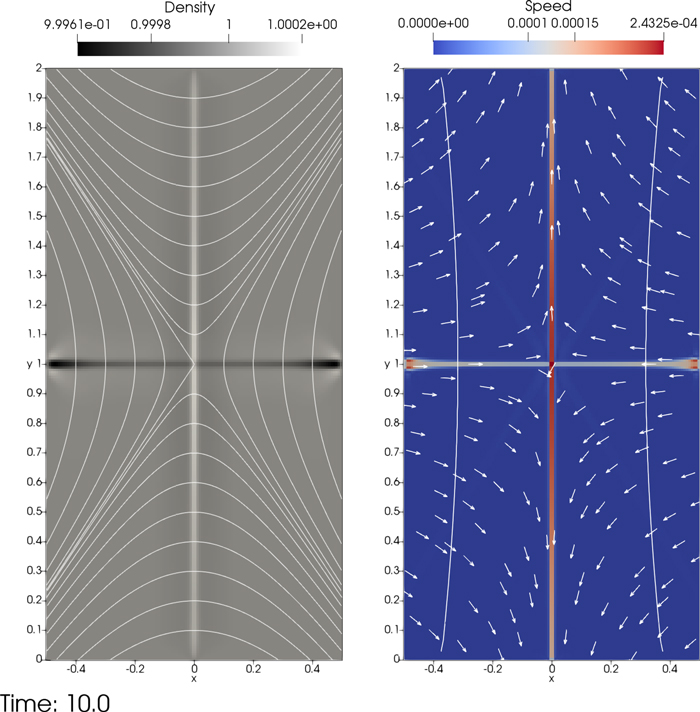
Figure 9. Density map with over-plotted magnetic field lines (left) and speed map with arrows indicating the local directions of Lorentz force (right) and solid lines where plasma  , at 10 time units with MFS in the 2D magnetic null-point test.
Download figure:
Standard image High-resolution imageAfter 10 time units (about 22,550 CFL limited time steps) in the MFS run, the density decreases at most 0.038% in the central horizontal line near the side boundaries and increases 0.02% in the central vertical line as shown in Figure 9, which corresponds to numerically generated diverging and converging flows to the horizontal and vertical line, respectively, with very small speeds of magnitude at most 2 × 10⁻⁴, which is only a 6 × 10⁻³ fraction of the local Alfvén speed. This cross-shaped pattern has only four cells in width. The reference run without MFS gives almost the same images as in Figure 9. The MFS run splits off the entire field above as  with its non-zero Lorentz force, and gives essentially the same results as the standard solver for the equilibrium state. We then perform a convergence study with increasing grid resolution, and plot kinetic energy, the ratio between kinetic energy and total energy, and magnetic energy normalized by its initial value at 10 time units in Figure 10. Both MFS runs and reference runs without MFS present very similar converging behavior and errors (deviations from the initial equilibrium) decrease with increasing resolution at fifthth order of accuracy. Therefore the correctness of the MFS technique for non-force-free fields is justified.

Figure 10. Kinetic energy (top panel), the ratio between kinetic energy and total energy (middle panel), and magnetic energy (bottom panel) normalized by its initial value at 10 time units for MFS runs (in circles) and reference runs (in plus) with different grid resolutions  , in the test presented in Section 3.2.2. Note the scale factor for the vertical axis in the bottom panel.
Download figure:
Standard image High-resolution image3.2.3. Current Sheet Diffusion
To test the MFS technique in resistive MHD, we first test dissipation of a straight current sheet with uniform resistivity. The magnetic field changes direction smoothly in the current sheet located at x = 0 as given by

Its current density is

In this test, we adopt parameter values Bd = 4 and current sheet width cw = 5. It is a nonlinear force-free field from a previous numerical study of magnetic reconnection of solar flares (Yokoyama & Shibata 2001). Initial density and gas pressure are uniformly 1.
We adopt a constant resistivity η with a dimensionless value of 0.1. The simulation box is 10 × 10 discretized on a four-level AMR mesh with an effective resolution of 512 × 512 cells. The average Alfvén crossing time is 2.5. After 1 time unit in an MFS run, the current is dissipated due to the resistivity as shown in panel (a) from Figure 11, presenting the z-component of current in rainbow color and magnetic field lines in gray scale. The Ohmic heating increases the temperature in the current sheet from 1 to 8, as shown in panel (b), with flows toward the current sheet from outside and velocity pointing outward in the heated current sheet as shown in panel (d). Plasma β ranges from 0.125 outside the current sheet and 4.2 in the middle of the current sheet. The reference run without MFS gives indistinguishable images as in Figure 11. To exactly compare the two runs, we evaluated the time evolution of magnetic energy, internal energy, and electric current and plot them in circles for MFS run and in triangles for the reference run in Figure 12. The results for the two runs almost overlap and the decrease of magnetic energy corresponds well to the increase of internal energy, this time by means of the adopted physical dissipation. We plot the normalized difference between them in the bottom panel, where within 0.1% differences are found for all three quantities. Therefore, the correctness of the MFS technique for resistive MHD is verified.

Figure 11. Dissipation of current sheet with MFS at 1 time unit. (a) z-component of electric current over-plotted with magnetic field lines colored by By. A purple line slicing across the current sheet is plotted with its temperature in (b), plasma β in (c), and vx in (d).
Download figure:
Standard image High-resolution image
Figure 12. Time evolution of (from top to bottom) magnetic energy, internal energy, and electric current in the case of MFS (in circles) and the non-split reference case (in triangles), in the test presented in Section 3.2.3. The very bottom panel quantifies their relative differences. Note the scale factor in the left top corner at each panel.
Download figure:
Standard image High-resolution image3.2.4. Solar Flare Application with Anomalous Resistivity
To show the advantage of the MFS technique in fully resistive settings, we present its application on a magnetic reconnection test which extends the simulations of solar flares by Yokoyama & Shibata (2001) to extremely low-β, more realistic situations. Here, a run without the MFS technique using our standard MHD solver fails due to negative pressure.
We set up the simulation box in ![$x\in [-10,10]$](https://content.cld.iop.org/journals/0067-0049/234/2/30/revision1/apjsaaa6c8ieqn119.gif) and
and ![$y\in [0,20]$](https://content.cld.iop.org/journals/0067-0049/234/2/30/revision1/apjsaaa6c8ieqn120.gif) with a four-level AMR mesh, which has an effective resolution of 2048 × 2048 and smallest cell size of 97 km. The magnetic field setup is the same current sheet as before, and follows Equation (38) with parameters Bd = 50 and cw = 6.667. Now, a 2D setup is realized with vertically varying initial density and temperature profiles as in Yokoyama & Shibata (2001), where a hyperbolic tangent function was used to smoothly connect a corona region with a high-density chromosphere. By neglecting solar gravity and setting constant gas pressure everywhere, the initial state is in an equilibrium. The current sheet is then first perturbed by an anomalous resistivity
with a four-level AMR mesh, which has an effective resolution of 2048 × 2048 and smallest cell size of 97 km. The magnetic field setup is the same current sheet as before, and follows Equation (38) with parameters Bd = 50 and cw = 6.667. Now, a 2D setup is realized with vertically varying initial density and temperature profiles as in Yokoyama & Shibata (2001), where a hyperbolic tangent function was used to smoothly connect a corona region with a high-density chromosphere. By neglecting solar gravity and setting constant gas pressure everywhere, the initial state is in an equilibrium. The current sheet is then first perturbed by an anomalous resistivity  in a small circular region in the current sheet when time
  , and afterwards the anomalous resistivity
  is switched to a more physics-based value depending on the relative ion–electron drift velocity. The formula of anomalous resistivity
  is
is

where  is the amplitude,
  is the distance from the center of the spot at
  , and
, and  is the radius of the spot. The formula of anomalous resistivity
  is
is

where  is the relative ion–electron drift velocity (e is the electric charge of the electron and n is number density of the plasma),
  is the threshold of the anomalous resistivity, and
  is the amplitude.
Continuous boundary conditions are applied for all boundaries and all variables except that Bx = 0 and zero velocity is imposed at the bottom boundary. We basically adopt the same setup and physical parameters as in Yokoyama & Shibata (2001), except that the magnitude of the magnetic field here reaches 100 G with plasma β of 0.005, compared to about 76 G and 0.03 in the original work. We use normalization units of length Lu = 10 Mm, time  , temperature
  K, number density
  cm−3, velocity vu = 116.45 km s−1, and magnetic field Bu = 2 G. Since we use different normalization units to normalize the same physical parameters, our dimensionless values are different from Yokoyama & Shibata's work. We choose a scheme combining HLL flux with van Leer's slope limiter (van Leer 1974) and two-step time integration. Powell's eight-wave method (Powell et al. 1999) is used to clean divergence of the magnetic field. Thermal conduction along magnetic field lines is solved using techniques that are described in detail in Section 4.
Inspired by Figure 3 in Yokoyama & Shibata (2001), we show very similar results in Figure 13, which presents snapshots of the density and temperature distribution at times 0.5, 0.64, and 0.75. The temporal evolution of the magnetic reconnection process and the evaporation in flare loops are reproduced. Flow directions and magnetic field lines are also plotted. Magnetic reconnection starts at the center x = 0, y = 6 of the enhanced resistive region, where an X-point is formed. Reconnected field lines with heated plasma are continuously ejected from the X-point to the positive and negative y-directions because of the tension force of the reconnected field lines.

Figure 13. Results of the solar flare simulation. Temporal evolution of density (top) and temperature (bottom) distribution. The arrows show the directions of velocity, and lines show the magnetic field lines integrated from fixed seed points at the bottom. Borders of AMR blocks are plotted in the density maps. Values in color bars are dimensionless.
Download figure:
Standard image High-resolution image4. Anisotropic Thermal Conduction
Thermal conduction in a magnetized plasma is anisotropic with respect to the magnetic field, as the thermal conductivity parallel to the magnetic field lines is much larger than that perpendicular to the field lines. This predominantly field-aligned heat flow can be represented by adding the divergence of an anisotropic heat flux to the energy equation. This heat source term can be numerically solved, independently of the MHD equations, using an operator splitting strategy. This means that we ultimately face the challenge of solving an equation due to anisotropic thermal conduction as:


where e is the internal energy  per unit volume, or it is the total energy density E from before. In this equation, T is temperature,
  is the (negative) heat flux vector, and
  is the unit vector along the magnetic field. The term
  represents the temperature gradient along the magnetic field.
  and
and  are conductivity coefficients for parallel and perpendicular conduction with respect to the local field direction. In most magnetized astronomical plasma,
  is dominant, for example in the solar corona, where
  is about 12 orders of magnitude smaller than
  . Therefore, we can typically ignore physical perpendicular thermal conduction, but we nevertheless implement both parallel and perpendicular thermal conduction for completeness. Note that when
  , the thermal conduction naturally degenerates to isotropic. In typical astronomical applications, we typically choose the Spitzer conductivity for
  erg cm−1 s−1 K−1.
4.1. Discretiziting the Heat Conduction Equation
To solve the thermal conduction Equation (42), various numerical schemes based on centered differencing have been developed. The simplest example is to evaluate gradients directly with second-order central differencing; more advanced methods include the asymmetric scheme described in Günter et al. (2005) and Parrish & Stone (2005) and the symmetric scheme of Günter et al. (2005). However, these schemes can cause heat to flow from low to high temperature if there are strong temperature gradients (Sharma & Hammett 2007), which is unphysical.
To understand why such effects can occur, consider Equation (42). Suppose a finite-volume discretization is used in 2D, and that we want to compute the heat flux in the x-direction at the cell interface between cell (i,j) and  . The term
  is then given by
  . The term
  will always be heat flux transported from hot to cold. When
  has the opposite sign of
  and a larger magnitude, a resulting unphysical heat flux from cold to hot occurs.
Avoiding the above problem, which can lead to negative temperatures, is especially important for astrophysical plasmas with sharp temperature gradients. Examples are the transition region in the solar corona separating the hot corona and the cool chromosphere, or the disk–corona interface in accretion disks. A solution was proposed in Sharma & Hammett (2007), in which slope limiters were applied to the transverse component of the heat flux. Since the slope-limited symmetric scheme was found to be less diffusive than the limited asymmetric scheme, we follow Sharma & Hammett (2007) and implement it in our code, with the extra extension to (temperature-dependent) Spitzer conductivity and generalized to a 3D setup in Cartesian coordinates. The explicit, conservative finite difference formulation of Equation (42) is then


involving face-centered evaluations of heat flux, e.g. along the x-coordinate, given by

in which  .
.
Since we use an explicit scheme for time integration, the time step  must satisfy the condition for numerical stability:

where cp is a stability constant taking value of 0.5 and 1/3 for 2D and 3D, respectively. With increasing grid resolution and/or high thermal conductivity, this limit on  can be much smaller than the CFL time step limit for solving the ideal MHD equations explicitly. Therefore multiple steps of solving thermal conduction within one-step MHD evolution are suggested to alleviate the time step restriction from thermal conduction. In our actual solar coronal applications, we adopt a super-timestepping RKL2 scheme proposed by Meyer et al. (2012), where every parabolic update uses an s-stage Runge–Kutta scheme with s and its coefficients determined in accord with the two-term recursion formula for Legendre polynomials. In what follows, we just concentrate on the details to handle a single step for the thermal conduction update.
The first term on the RHS of expression (46) is discretized as the limited face-centered heat flux:

where the local thermal conduction coefficient is found by first quantifying its value at the cell corners, in 3D ( ) found from

to then derive the face-centered values as in

The face-centered, limited flux expression is given by

in which corner values for the magnetic field aligned unit vectors are found as in

while the limited temperature gradient in cell corners is found from


Similar formulae (involving fewer summations in the averaging) apply at lower dimensionality  . We choose
  for 2D runs, the same value as used by Sharma & Hammett (2007), and
  for 3D runs to achieve least numerical diffusion according to our trial-and-error numerical tests. Note that in our code, as assumed in the above, the magnetic field components (and other quantities, like temperature) are defined at cell centers, and different formulae would be needed for a staggered grid where magnetic field is defined at cell faces, such as commonly adopted in constrained transport schemes.
The second and third terms of Equation (46) are transverse components qxy and qxz of heat conduction; we illustrate the discretization of the second term here and the third term can be derived similarly:

where  and
and  follow the same formula as Equation (50) for
  . The limited, face-centered temperature gradient is evaluated as in

in which

where  is the monotonized central (MC) slope limiter, which is given by

We have tried other slope limiters such as minmod, vanleer, and superbee, but MC limiter gives the best results.
The last term of Equation (46) contributes to perpendicular thermal conduction and its discretized form computes the averaged face value of  using the same form as Equation (50) and the averaged face value of the temperature gradient along x as in Equation (51) (and the equations that follow it), but without the factors bx2.
Since thermal conduction in dilute plasmas is caused by the movement of electrons, a larger thermal conduction flux implies faster electrons. Once the electron speed becomes comparable to the sound speed, plasma instabilities prevent the electrons from flowing faster and thermal conduction must saturate (Cowie & McKee 1977). We adopt the following formula from Cowie & McKee (1977) for a saturated thermal flux:

where  is the isothermal sound speed and the factor
  when the electron and ion temperatures are equal. We evaluate the projected saturated thermal flux at each cell face based on the averaged density and temperature there, and set it as the upper limit for the total thermal flux through that cell face, namely,
  .
.
We implement the methods mentioned above in a thermal conduction module with source code written in the dimension-independent LASY way. Thus the same compact source code can be translated to pure Fortran code in 1D, 2D, or 3D before compilation.
4.2. Anisotropic Heat Conduction Test Problems: 2D to 3D
A 2D circular ring diffusion test problem was proposed by Parrish & Stone (2005) and became a standard test for anisotropic thermal conduction (Sharma & Hammett 2007; Meyer et al. 2012). It initializes a hot patch in circular magnetic field lines in a ![$[-1,1]\times [-1,1]$](https://content.cld.iop.org/journals/0067-0049/234/2/30/revision1/apjsaaa6c8ieqn168.gif) Cartesian box with temperatures
Cartesian box with temperatures

where  and
and  . Density is set to 1. We create circular magnetic field lines centered at the origin by the formula:

which is generated by an infinite line current perpendicular to the plane through the origin. The parallel thermal conductivity is constant and set to  and no explicit perpendicular thermal conduction is considered. Continuous boundary conditions are used for all variable at all boundaries. We only evolve the anisotropic thermal heat conduction equation without solving the MHD equations, until 400 time units. Ideally, the diffusion of temperature should only occur in a ring
  and eventually result in a uniform temperature of 10.1667 inside the ring with unperturbed temperature of 10 outside the ring. But perpendicular numerical diffusion may cause some cross-field thermal conduction and can smooth sharp temperature gradients at the borders of this ring.
The end state of a run (a) on a uniform 200 × 200 grid is shown in Figure 14(a). Temperature is high and nearly uniform inside the ring, with a constant background temperature of 10. The maximal and minimal temperature of the end state are 10.1687 and 10, respectively. No temperature overshooting is found near sharp temperature gradient regions and the monotonicity property is preserved. The final temperature distribution agrees with previous findings (see the fourth panel in Figure 6 of Sharma & Hammett 2007). Since the exact solution of this problem is a uniform temperature of 10.1667 in the ring and 10 outside it, we can evaluate the L1, L2, and  norm errors for four runs with increasing resolution (see Table 1). The L1 norm converges with a rate of 1.4 and the L2 norm converges with a rate of 0.8. The maximal temperature is getting closer to the correct solution with increasing resolution and the minimal temperature stays at the correct value of 10. A rough estimate for the time-averaged perpendicular numerical diffusion (conductivity)
  and its ratio to
  are calculated following the same method as in Sharma & Hammett (2007), and reported in the last column of Table 1. Note in particular that we can get this ratio from order 10−3 down to order 10−5 on sufficiently large grids, so that we can add physical perpendicular thermal conduction coefficients that exceed these values.

Figure 14. Temperature at 400 time units for four cases initialized with the ring diffusion problem: (a) on a uniform 200 × 200 grid; (b) on an AMR grid with 200 × 200 effective resolution; (c) the same condition as (a) except that perpendicular conduction with  is included; (d) the same condition as (b) except for excluding conservation fix.
Download figure:
Standard image High-resolution imageTable 1. Accuracy Measures of the Ring Diffusion Tests on Uniform Grids
| Resolution | L1 error | L2 error |
 error error |

|

|

|
|---|---|---|---|---|---|---|
| 50 × 50 | 0.03037 | 0.04705 | 0.08617 | 10.0842 | 10 |

|
| 100 × 100 | 0.01338 | 0.02704 | 0.11654 | 10.1355 | 10 |

|
| 200 × 200 | 0.00521 | 0.01592 | 0.08683 | 10.1663 | 10 |

|
| 400 × 400 | 0.00320 | 0.01224 | 0.08758 | 10.1681 | 10 |

|
Download table as: ASCIITypeset image
In order to use the thermal conduction on an AMR grid, refluxing operations are needed to ensure flux conservation across fine–coarse interfaces. We store the thermal fluxes of blocks with finer or coarser neighbor blocks, and send thermal fluxes at fine–coarse interfaces from finer blocks to coarser blocks. This is standard practice for ensuring conservation in finite-volume AMR computations, and our strategy in terms of parallel communication patterns involved is found in Section 3.4 of Keppens et al. (2012). Figure 14(b) shows the end state of run (b) on an AMR grid with three levels and an effective resolution of 200 × 200. We use dynamic AMR, with the refine-triggering based on total energy using a Löhner type estimator (Lohner 1987; Keppens et al. 2012) and set a refine threshold of 0.08. Comparing to the result of the run in panel (a) on a uniform grid with the same resolution, run (b) gives comparable results. The AMR advantage is in the fact that it uses about 20% less computational time. Some minor quality degeneracy is present, with less sharp borders of the ring segment at the far end from the initial hot segment and a lower maximal temperature of 10.1638. This is likely caused by the larger numerical diffusion associated with the coarser grids at the far end. To prove the importance of the conservation fix, we show a run (d) with the same setup as run (b), except that it has no conservation fix, which ends up with lower temperature in the ring and stronger diffusion at its borders, as shown in Figure 14(d). To test our implementation of perpendicular thermal conduction, we perform test run (c) with a constant  and other setups the same as run (a). As shown in Figure 14(c), the parallel thermal conduction dominates the diffusion of initial temperature pattern while finite perpendicular thermal conduction significantly smoothed the hot ring pattern in the radial direction of the ring perpendicular to magnetic field lines, comparing to run (a). The test run (c) demonstrates the correctness of our implementation of perpendicular thermal conduction, which may become non-negligible in plasma with very weak magnetic field.
We generalize the 2D ring diffusion test to a 3D version. In a 3D ![${[-1,1]}^{3}$](https://content.cld.iop.org/journals/0067-0049/234/2/30/revision1/apjsaaa6c8ieqn186.gif) Cartesian box, we rotate the magnetic field loops, from a position at first in the x–y plane, around the x-axis 45°, and then rotate around the z-axis 45°, to make the magnetic field direction misaligned with the coordinates. Therefore, the thermal flux along magnetic field lines must include contributions from all three dimensions. An initial 3D hot patch is set to have the same extension in the plane of the magnetic loop as in the 2D case and an extension of 0.4 in the direction perpendicular to this plane. We run the test on a uniform
Cartesian box, we rotate the magnetic field loops, from a position at first in the x–y plane, around the x-axis 45°, and then rotate around the z-axis 45°, to make the magnetic field direction misaligned with the coordinates. Therefore, the thermal flux along magnetic field lines must include contributions from all three dimensions. An initial 3D hot patch is set to have the same extension in the plane of the magnetic loop as in the 2D case and an extension of 0.4 in the direction perpendicular to this plane. We run the test on a uniform  mesh until 400 time units. As shown in Figure 15(a), the 3D isosurface of temperature at 10.16 represents a ring shape. A slice through the middle plane of the ring structure is shown in a warped view and colored by temperature in Figure 15(b), and is comparable with the previous 2D results. The maximal temperature in the hot ring of the slice is 10.1774 and its thickness is 10% larger than in the corresponding 2D tests. A translucent slice cutting through the ring in panel (a) shows, in panel (c), that its cross section has a rounded square shape, which is caused by large numerical diffusion at its corner edges. To test the 3D thermal conduction on an AMR mesh, we run the same 3D test problem on a three-level AMR mesh with base-level resolution of
  , which has the same effective resolution as the previous test on a uniform mesh. The result is very similar to the uniform-mesh version with maximal temperature of 10.1727, while the run consumes 45% less computational time than the uniform-mesh run.
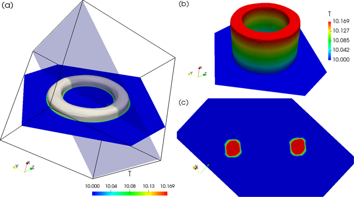
Figure 15. Temperature at 400 time units in a 3D case initialized with the ring diffusion problem on a uniform  grid. (a) Isosurface of temperature at 10.16 and a plane slicing through the middle of the hot patch in the 3D box; (b) 3D view of the 2D slice plane in (a), warped and colored by temperature; (c) temperature on the translucent slice in (a).
Download figure:
Standard image High-resolution imageTo check the consistency between the 3D implementation and the 2D one, we set up a test of 2D ring diffusion problem in a 3D simulation. We set the magnetic field loops in the x–y plane and the initial hot patch has the same extension in the x and y directions as in the 2D setup and extends uniformly through the box in the z direction. Periodic boundary conditions are used at z boundaries and continuous boundary conditions are adopted at x and y boundaries. The simulation box has a size of 1 × 1 by 0.1 on a  mesh. The temperature distribution is invariant in the z direction and its x–y plane slice is very close to the 2D result with the same resolution at 400 time units. The maximum and miminum temperatures are the same. The temperature transition region is about 4% broader in the 3D run. Therefore, the 3D implementation is consistent with the 2D one.
5. Performance and Scaling
In the previous version of MPI-AMRVAC, the root-level blocks were connected with a simple dimension-by-dimension incremental order curve, while a Morton-ordered space filling curve was recursively applied from level 2 onwards, refining root level blocks, to the leaf levels (Keppens et al. 2012). In MPI-AMRVAC 2.0, we also connect the root-level blocks with a Morton-ordered space-filling curve, as illustrated in Figure 16, to improve data locality and minimize times of inter-processor communications. Since a pure Morton curve connects nodes arranged in a square shape in 2D or in a cubic shape in 3D which have the same even number of node blocks along each dimension, we cannot directly apply it to a domain with nodes arranged in a non-square shape or with odd number of node blocks. In a true rectangular case, e.g., 5 × 2 in Figure 16, we first extend the rectangular domain to a square one, namely 6 × 6, apply the standard Morton curve on it, and remove nodes that lie outside of the rectangular domain. To remove a node on a space-filling curve, we simply delete the node and subtract one from the numbers of all nodes behind it. In addition to that, we further reduce communication by skipping the communication and update of corner cells, if they are not needed in a certain physics solver. Optimizations include speeding up the flux calculation, avoiding using split source terms which need an extra ghost cell update by communication, and minimizing the conversion between primitive and conservative variables, (e.g., providing both primitive and conservative left and right state at cell interfaces after reconstruction for flux evaluation).

Figure 16. Morton-ordered curve illustrated for a rectangular domain with 5 × 2 root level blocks.
Download figure:
Standard image High-resolution imageWith this new block ordering, we present two sets of tests to demonstrate strong scaling of MPI-AMRVAC on BrENIAC, the Flemish Tier-1 supercomputer. The first one is solving a 3D blast wave problem in ideal MHD physics. The simulation box is of size 2 × 2 × 2 on a uniform mesh of 5123 cells. The mesh is decomposed into 323 blocks with each block of 163 cells. Initially, gas pressure is 100 inside a central ball with radius of 0.2 and 1 outside, density is uniformly 1, magnetic field is uniform with  , and velocity is zero. We use the same schemes as explained at the beginning of Section 3.2, namely, HLL flux, Čada's compact third-order limiter, the three-step Runge–Kutta time integration, and the diffusive approach to clean divergence of magnetic field. To do a strong scaling test, we run the same test with increasing number of cores, starting from 28 cores to 3584 cores. We plot speed as cells updated per second and efficiency of speed-up in Figure 17, where the black line shows ideal scaling with 100% efficiency. The runs with the previous code version MPI-AMRVAC 1.0, plotted as empty triangles, stop speeding up after 1729 cores, while the new MPI-AMRVAC 2.0, plotted as dots, shows much better scaling. When running on 3584 cores (37,449 cell per core), the test with MPI-AMRVAC 2.0 still has 54% speed-up efficiency with respect to the speed of 28 cores. Note that each data point reported here is an average result of three repeated runs.

Figure 17. Strong scaling of an ideal MHD application with a 5123 cell uniform mesh for MPI-AMRVAC 2.0 shown as dots and for MPI-AMRVAC 1.0 shown as empty trangles. (a) Cells updated per second for increasing number of cores. The solid line shows the ideal scaling case. (b) Efficiency of the speed-up, shown as a function of the number of cells per core.
Download figure:
Standard image High-resolution imageThe second test comes from an actual solar application, where we have done a 3D coronal rain dynamics simulation (Xia et al. 2017), which solves MHD coupled with parameterized heating, optically thin radiative cooling, and anisotropic thermal conduction as described in Section 4. We used an AMR mesh to resolve high-density, low-temperature coronal rain blobs when they form and fall down in a magnetic arcade (Xia et al. 2017). The AMR mesh is composed of 123-cell (excluding ghost cells) blocks organized in five AMR levels. To do this strong scaling test, we take a snapshot (at time 46.3 min) from this coronal rain simulation, restart the simulation from that moment, and run for 10 time steps, with one data output at the end. About 46.4 million cells in 26,652 blocks are evolved. AMR mesh is re-evaluated for (de)refinement every three time steps, although ultimately the mesh structure and number of blocks do not change during the test. We use the same schemes as in the first test and the MFS technique mentioned in Section 3. The results of a strong scaling test are shown in Figure 18. More than 60% efficiency is obtained when using up to about 2000 cores, with more than 5 × 10⁴ cells per core.
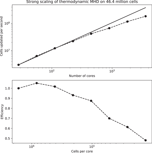
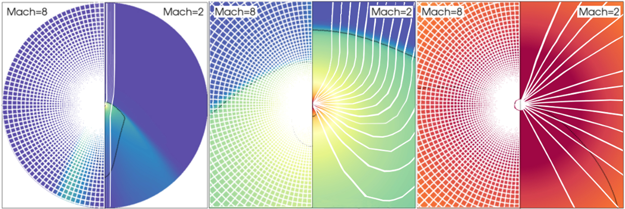
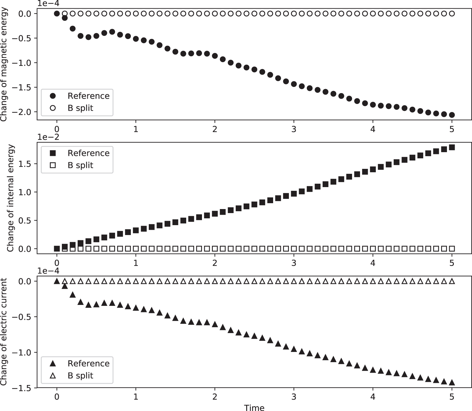
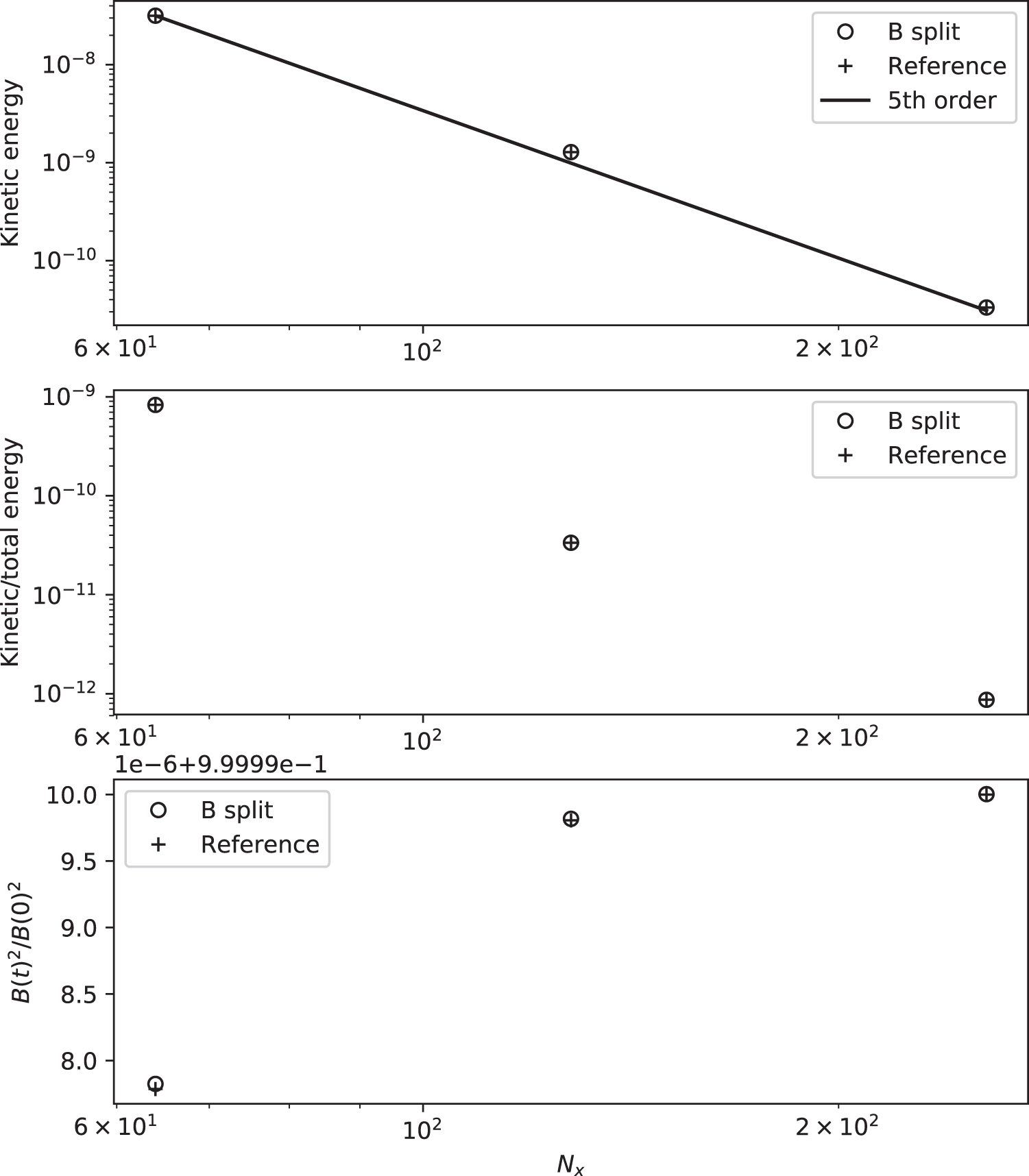
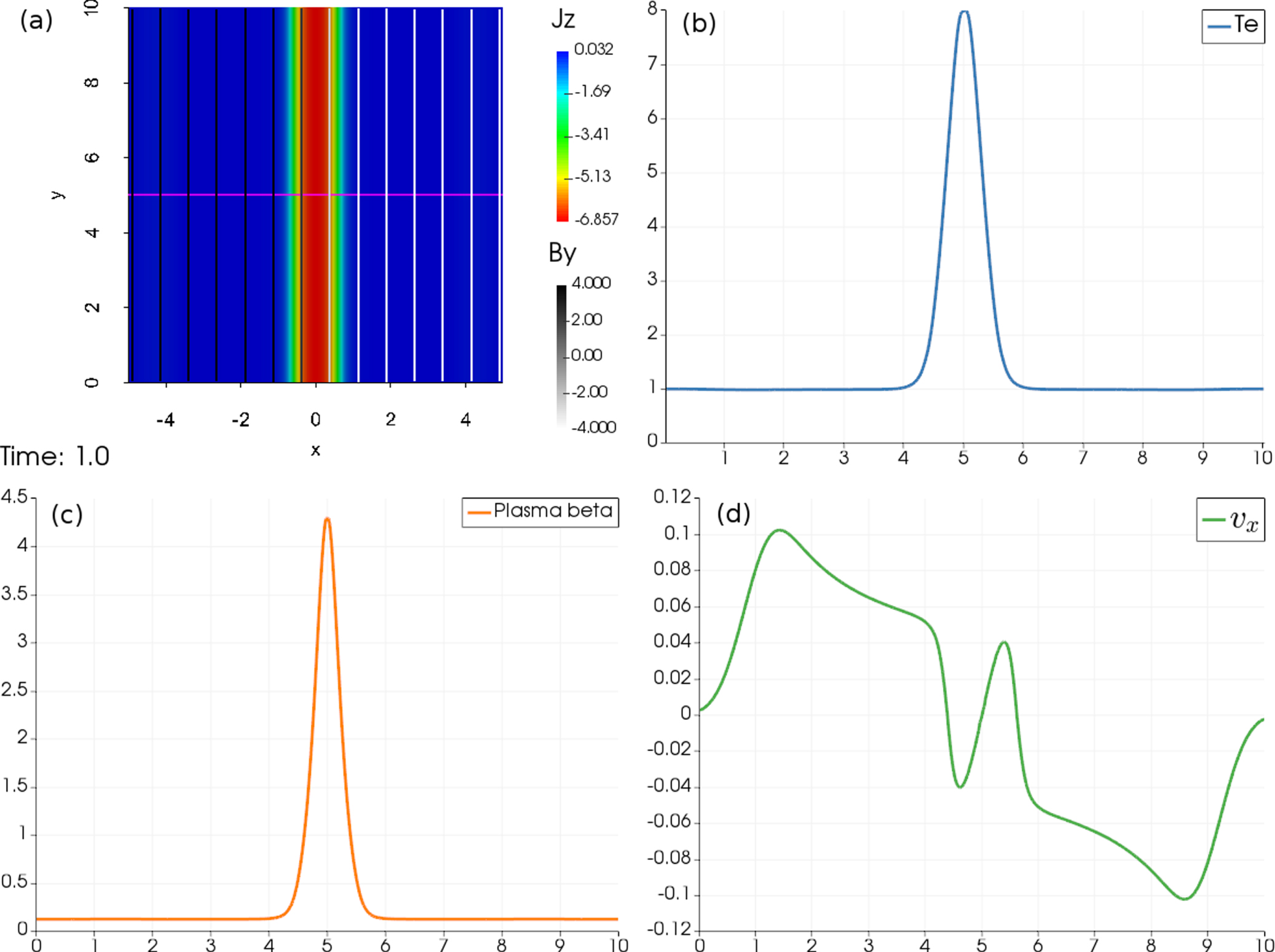
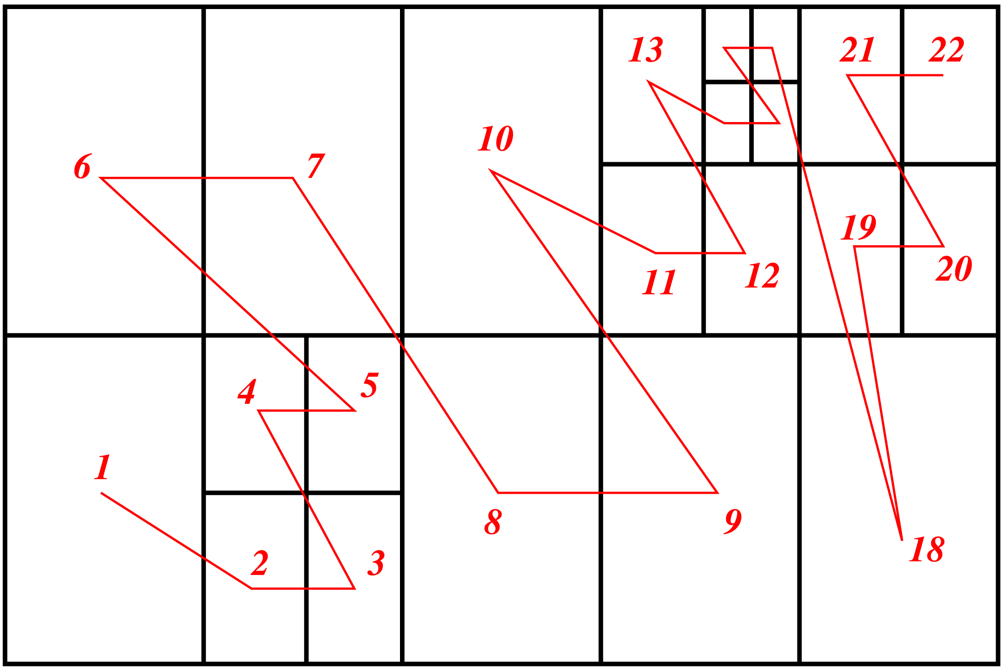
Figure 18. Strong scaling of a thermodynamic AMR-MHD application with 46.4 million cells. (a) Cells updated per second for increasing number of cores in dots connected with a dashed line. The solid line shows the ideal scaling. (b) Efficiency of the speed-up, shown as a function of the number of cells per core.
Download figure:
Standard image High-resolution image
6. Generic Framework Improvements
MPI-AMRVAC has been in development since early this century (Nool & Keppens 2002), and many scientists contributed code to it. These contributions usually aimed to enable new research, for example by adding numerical methods or extending physics models. In the most recent restructuring effort, we modernized the underlying framework, which we hope will help in maintaining and developing the framework in the decades to come. In this section, we describe improvements we made in this regard.
6.1. Modernization of the Framework
MPI-AMRVAC is written in Fortran extended by the LASY syntax (Tóth 1997). After source files have been translated by a LASY preprocessor, they can be compiled by a standard Fortran compiler. The main goal of the LASY syntax is to be able to write dimension-independent code. However, the LASY syntax was also used, for example, to:
- 1.(optionally) include other source files,
- 2.perform vectorization (e.g., loop over components),
- 3.define parameters for specific applications,
- 4.turn parts of the code on or off.
This extended use of the preprocessor made it harder to understand the code, especially as more and more features were added. The preprocessor in MPI-AMRVAC 2.0 has therefore been simplified; the only flags it now supports relate to the dimensionality of the problem. Hence, the preprocessor is now only used to translate dimension-independent code to 1D, 2D, or 3D. This simplification of the preprocessor also required another modernization: instead of source files that were optionally included as flags were turned on or off, we now make use of standard Fortran modules. This made it possible to compile the full framework into a static library, including all the physics modules at once. This helps to ensure code stays compatible (and compiles) whenever changes are made, and significantly reduces compilation times. Furthermore, parallel compilation is now supported.
The modifications imply that the user program now has to specify which type of major physics module to activate, for example the hydrodynamics or MHD one (previously handled through the preprocessor and before compilation). As all modules are now available in the library version, this raises awareness of users to the full framework functionality, and each physics module now comes with its own settings and parameters, for example whether or not an energy equation should be used, or how many tracers (or dust species in coupled gas-dust hydro problems) to be included. Thanks to that, users can switch on/off special functionalities, like thermal conduction, radial stretching grid, particles etc., by just choosing appropriate parameters in an input parameter file without wasting time on recompilation, which was needed more frequently in the old code. Furthermore, we provide extensive support for customization to a large variety of applications by using function pointers. A user has to provide a routine for setting initial conditions, but can also specify custom routines for boundary conditions, additional source terms, custom output routines etc. There have also been many smaller changes to help users, most importantly those related to handling the coordinate system explicitly (by selecting, e.g., Cartesian 2D or 2.5D, or cylindrical, polar up to spherical 3D). Methods are encoded to automatically use the right number of ghost cells, and the MPI-AMRVAC 2.0 settings to run an actual application can now be specified in multiple parameter files.
6.2. Automatic Regression Tests
A very important addition concerns regression tests for MPI-AMRVAC, in which their output is compared to stored "correct" results. We intend to have a least one such test for each type of major functionality that the code supports, varying dimensionality, equations to solve, or choice of algorithmic approach. The primary goal of these tests is to ensure that code changes do not affect the result of existing simulations. They can also help new users to explore MPI-AMRVAC's functionality, and to detect bugs and incompatibilities.
The implementation of these tests is as follows. First, a standard simulation is scaled down so that it can be run in a short time, e.g., one to ten seconds on a standard machine. We then specify the program to produce a log file of type "regression_test," which contains  and
and  over time, where
  is a vector of the nw (typically conservative) physical variables wi per cell, for all variables
 ![$i\in [1,{n}_{w}]$](https://content.cld.iop.org/journals/0067-0049/234/2/30/revision1/apjsaaa6c8ieqn195.gif) . By comparing both the volume-integrated values of both cell values and their squares, errors in conservation properties and almost all errors in the shape of the solution are detected. The resulting log file is then compared to a previously stored version, using a finite error threshold in comparing values a to b as in:
. By comparing both the volume-integrated values of both cell values and their squares, errors in conservation properties and almost all errors in the shape of the solution are detected. The resulting log file is then compared to a previously stored version, using a finite error threshold in comparing values a to b as in:

where we by default use an absolute tolerance of  and relative tolerance of
  . These tolerances account for changes due to numerical roundoff errors. Roundoff errors can for example occur when computations are re-ordered (using different compilation flags and/or compilers) or when a different number of processors is used. Most of the tests we have are performed for several combinations of numerical schemes. They can be executed automatically by running "make" in the tests folder of MPI-AMRVAC.
6.3. Doxygen Documentation
Having good documentation can increase the efficiency of both users and maintainers. However, as it takes considerable effort to write such documentation, this remains an ongoing process. For new contributions, we follow these guidelines for inline documentation:
- 1.provide a short description of a non-trivial function/subroutine,
- 2.when a piece of code is hard to understand, briefly describe what it does,
- 3.variable names should be self-explanatory without getting lengthy.
For MPI-AMRVAC 2.0 we make use of Doxygen (see http://www.doxygen.org), so that most documentation can be written close to the code it documents. This helps when reading the code, but also makes it simpler to update documentation when changing code. The documentation is automatically generated every day and published on http://amrvac.org, which provides a starting point for new users.
6.4. New Binary Format
MPI-AMRVAC can write output in several visualization formats, such as VTK or Tecplot. Furthermore, there is support for binary output files. These files can be used to restart a simulation, or to convert simulation data to any of the supported visualization file formats. For MPI-AMRVAC 2.0, we revised this binary format to make it future proof and simpler to use. The new binary format has a relatively simple structure, see Table 2, and it can be read and written with a modest amount of Fortran (or Python, C, etc.) code. Some of the changes with regards to the old format are:
- 1.the introduction of a version number to provide backwards functionality,
- 2.the header is now at the start of the file, to simplify reading files,
- 3.byte offsets pointing to the location of the tree information and the block data allow new variables to be added at the end of the header,
- 4.for each block, we also store its refinement, spatial index in the grid, and the location of its data, to facilitate reading in data,
- 5.each grid block can now also store ghost cells.
Table 2. Description of the file Format for Binary Files, in Order of Appearance in the File
| Description | Variable Name | Data Type |
|---|---|---|
| Header | ||
| Version number | int32 | |
| Offset tree info | int32 | |
| Offset block data | int32 | |
| Number of variables | nw | int32 |
| Dimension of vectors | ndir | int32 |
| Dimension of grid | ndim | int32 |
| Maximum refinement level | int32 | |
| Number of grid leaves | nleafs | int32 |
| Number of grid parents | nparents | int32 |
| Time iteration count | int32 | |
| Simulation time | float64 | |
| Min. coordinates | float64(ndim) | |
| Max. coordinates | float64(ndim) | |
| Resolution of base-level mesh | domain_nx | int32(ndim) |
| Resolution of a block | block_nx | int32(ndim) |
| Geometry name | character(16) | |
| Names of variables | character(nw*16) | |
| Name of physics | character(16) | |
| Number of physics parameters | nparams | int32 |
| Parameters | float64(nparams) | |
| Parameter names | character(nparams*16) | |
| Tree information | ||
| Leaf or parent | logical(nleafs+nparents) | |
| Refinement level | int32(nleafs) | |
| Spatial index | int32(ndim * nleafs) | |
| Block offset | int64(nleafs) | |
| Block 1 | ||
| Number of lower ghost cells | glo | int32(ndim) |
| Number of upper ghost cells | ghi | int32(ndim) |
| Block data | float64(1-glo:block_nx+ghi, nw) | |
| Block 2 | ||
| ... | ||
Download table as: ASCIITypeset image
We remark that the use of a format such as HDF5 would offer advantages in terms of standardization and portability. However, this would add a dependency on HDF5, which could complicate code installation and compilation for users and would require all our current tools for binary files to be rewritten.
7. Conclusions and Outlook
We provide an update on the open source software MPI-AMRVAC (Porth et al. 2014c), suited for parallel, grid-adaptive computations of hydrodynamic and MHD astrophysical applications. Motivated by recent applications in the context of transonic accretion flows onto compact objects, or trans-Alfvénic solar wind outflows, we combine grid stretching principles with block-adaptivity. Its advantage is demonstrated in 1D, 2D, and 3D scenarios, on spherically symmetric Bondi accretion, steady planar Bondi–Hoyle–Lyttleton flows, 3D wind accretion in supergiant X-ray binaries, and 2D solar wind. In especially solar physics-oriented MHD applications, we show the benefits of a generalization of the original potential magnetic field-splitting approach, which allows splitting off any magnetic field. This is demonstrated in tests with a 3D static force-free magnetic flux rope, in settings with a 2D magnetic null-point, and in resistive MHD scenarios about magnetic reconnection in current sheets with either uniform or anomalous resistivity. The latter revisits a pioneering solar flare application with inclusion of anisotropic thermal conduction by Yokoyama & Shibata (2001), which can now be simulated at more realistic low plasma beta conditions. We provide details on our implementation for treating anisotropic thermal conduction in multi-dimensional MHD applications, generalizing slope-limited symmetric schemes by Sharma & Hammett (2007) from 2D to 3D configuration, and ring diffusion tests that demonstrate its high accuracy and robustness in preventing unphysical thermal flux from which all traditional schemes cannot avoid. The new version of the code is shown to scale much better than the old one and its strong scaling is satisfactory up to 2000 cores in AMR simulations on 3D solar coronal rain driven by thermal instabilities. Generic improvements are also reported: modularization and monolithic compilation into a static library, the handling of automatic regression tests, the use of inline/online Doxygen documentation, and a new future-proof data format for input/output and restarts of simulations.
MPI-AMRVAC 2.0 is freely available on http://amrvac.org, and can be used for a fair variety of hydrodynamic to MHD computations. In a forthcoming paper (B. Ripperda et al. 2018, in preparation), we will document the code capability to solve for particle dynamics using a variety of solvers for handling the governing Lorentz equation, or by using a set of ordinary differential equations for quantifying their gyro-averaged motion. This can be done in static, as well as in dynamic, electromagnetic fields obtained from MHD applications, as recently demonstrated in Ripperda et al. (2017a, 2017b). In combination with the capabilities documented in this paper, these improvements prepare for future applications of violent solar eruptive phenomena, and the reconnection physics and particle acceleration associated with them. In the longer term, we envision handling Poisson problems on the AMR hierarchy, or improving the treatment of radiative losses beyond the simplistic optically thin assumption.
C.X., J.T., I.E.M., and E.C. wish to thank FWO (Research Foundation Flanders) for the award of a postdoctoral fellowship to them. This research was supported by FWO and by KU Leuven Project No. GOA/2015-014 and by the Interuniversity Attraction Poles Programme by the Belgian Science Policy Office (IAP P7/08 CHARM). The simulations were conducted on the VSC (Flemish Supercomputer Center funded by Hercules foundation and Flemish government).
Software: MPI-AMRVAC 2.0 (Xia et al. 2018), MPI-AMRVAC 1.0 (Porth et al. 2014c).