
APPENDIX C
Design Example 1 — Embankment Fill Over Clay Using Hand Calculations
Design Example Problem 1 was formulated from the Briaud and Tucker (1997) Example Problem 1, as found on Pages 99 through 101 of Briaud and Tucker (1997). The data sheets (Pages 86 through 88 of Briaud and Tucker, 1997), that were used to program the data into the Briaud and Tucker (1997) PILENEG program, were referenced for the Design Example Problem 1 that is presented herein. Procedures for determining the location of the neutral plane and magnitudes of the drag load and downdrag are demonstrated using 1) Load-Resistance profiles and 2) Pile-Soil Settlement profiles by means of the proposed Method A (fully-mobilized) procedures proposed by the NCHRP 12-116A project team. This design example is related to pile loading resulting from a change in effective stress in the soil deposit due to an embankment load being placed on the soil surface. The example is provided through a series of steps to aid in completion of the analysis. The series of steps follow the flowchart proposed by the NCHRP 12-116A project team. For clarity, the modified series of procedural steps follow the NCHRP12-116A flowchart that is shown on the next page instead of the steps that were provided on pages 59 through 63 of Briaud and Tucker (1997). The design example is presented in SI units because the original Briaud and Tucker (1997) data were in SI units.
The provided data included the maximum shaft resistance and pile shape, cross-sectional area, embedded length, and modulus (Pages 85 and 87 of Briaud and Tucker, 1997). The load placed at the top pile was also provided (Page 86 of Briaud and Tucker, 1997). Additional information included soil settlement data and soil bearing data including Young’s modulus, Poisson’s ratio, and the ultimate bearing resistance (Page 88 of Briaud and Tucker, 1997). The provided data are summarized in Table C1. The output data from the PILENEG program, as found on pages 99-100 of Briaud and Tucker (1997), are presented in Table C2.
Table C1. Briaud and Tucker (1997) Example Problem 1 PILENEG Program input data.
| Pile Material | Concrete | * Inferred or interpolated parameters using correlations contained in Briaud and Tucker (1997). Fig. 2.5 in this table refers to Fig. 2.5 from Briaud and Tucker (1997). | |
| Pile Shape | Octagonal | ||
| Pile Face [mm] | 174* | ||
| Pile Perimeter [m] | 1.39 | ||
| Pile Area [m2] | 0.145 | ||
| Pile Embedded Length [m] | 41.76 | ||
| Pile Modulus [kN/m2] | 2.41 x 10⁷ | ||
| Top Load on Pile [kN] | 2225 | ||
| Number of Pile Increments | 50 | ||
| Maximum Shaft Resistance | Depth [m] | Shaft Resistance [kN/m2] | |
| 0 | 12.92, 13*(su B&T Fig. | ||
| 22.86 | 30.80, 31*(su B&T Fig. | ||
| 41.76 | 94.18, 128* (su Fig. 2.5) | ||
| Soil Settlement | Depth [m] | Soil Settlement [m] | |
| 0 | 0.335 | ||
| 6.10 | 0.165 | ||
| 9.14 | 0.119 | ||
| 12.19 | 0.088 | ||
| 15.24 | 0.058 | ||
| 21.34 | 0.034 | ||
| 41.76 | 0.015 | ||
| Soil Young’s Modulus [kN/m2] | 21531 | ||
| Soil Poisson’s Ratio | 0.3 | ||
| Soil Ultimate Bearing Capacity | 7097 | ||
| Groundwater Table Depth [m] | 0* |

Table C2. Briaud and Tucker (1997) Example Problem 1 PILENEG Program output data.
| Depth [m] | Axial Force [kN] | Axial Stress [kN/m2] | Soil Settlement [m] | Pile Settlement [m] |
| 0.000E+00 | 2.225E+03 | 1.534E+04 | 3.200E-01 | 9.047E-02 |
| 8.352E-01 | 2.240E+03 | 1.545E+04 | 2.967E-01 | 8.994E-02 |
| 1.670E+00 | 2.257E+03 | 1.556E+04 | 2.734E-01 | 8.940E-02 |
| 2.506E+00 | 2.273E+03 | 1.568E+04 | 2.502E-01 | 8.886E-02 |
| 3.341E+00 | 2.291E+03 | 1.580E+04 | 2.269E-01 | 8.831E-02 |
| 4.176E+00 | 2.309E+03 | 1.593E+04 | 2.036E-01 | 8.776E-02 |
| 5.011E+00 | 2.329E+03 | 1.606E+04 | 1.803E-01 | 8.721E-02 |
| 5.846E+00 | 2.349E+03 | 1.620E+04 | 1.571E-01 | 8.665E-02 |
| 6.682E+00 | 2.369E+03 | 1.634E+04 | 1.412E-01 | 8.609E-02 |
| 7.517E+00 | 2.391E+03 | 1.649E+04 | 1.286E-01 | 8.552E-02 |
| 8.352E+00 | 2.413E+03 | 1.664E+04 | 1.159E-01 | 8.494E-02 |
| 9.187E+00 | 2.436E+03 | 1.680E+04 | 1.035E-01 | 8.436E-02 |
| 1.002E+01 | 2.460E+03 | 1.696E+04 | 9.503E-02 | 8.378E-02 |
| 1.086E+01 | 2.484E+03 | 1.713E+04 | 8.654E-02 | 8.319E-02 |
| 1.169E+01 | 2.509E+03 | 1.731E+04 | 7.805E-02 | 8.259E-02 |
| 1.253E+01 | 2.535E+03 | 1.748E+04 | 6.968E-02 | 8.199E-02 |
| 1.336E+01 | 2.527E+03 | 1.743E+04 | 6.146E-02 | 8.138E-02 |
| 1.420E+01 | 2.500E+03 | 1.724E+04 | 5.325E-02 | 8.078E-02 |
| 1.503E+01 | 2.472E+03 | 1.705E+04 | 4.503E-02 | 8.019E-02 |
| 1.587E+01 | 2.443E+03 | 1.685E+04 | 4.053E-02 | 7.960E-02 |
| 1.670E+01 | 2.413E+03 | 1.664E+04 | 3.724E-02 | 7.902E-02 |
| 1.754E+01 | 2.382E+03 | 1.643E+04 | 3.395E-02 | 7.845E-02 |
| 1.837E+01 | 2.351E+03 | 1.621E+04 | 3.067E-02 | 7.788E-02 |
| 1.921E+01 | 2.319E+03 | 1.599E+04 | 2.738E-02 | 7.732E-02 |
| 2.004E+01 | 2.286E+03 | 1.577E+04 | 2.410E-02 | 7.677E-02 |
| 2.088E+01 | 2.253E+03 | 1.553E+04 | 2.081E-02 | 7.623E-02 |
| 2.172E+01 | 2.218E+03 | 1.530E+04 | 1.865E-02 | 7.570E-02 |
| 2.255E+01 | 2.183E+03 | 1.506E+04 | 1.787E-02 | 7.517E-02 |
| 2.339E+01 | 2.146E+03 | 1.480E+04 | 1.710E-02 | 7.465E-02 |
| 2.422E+01 | 2.107E+03 | 1.453E+04 | 1.632E-02 | 7.414E-02 |
| 2.506E+01 | 2.064E+03 | 1.424E+04 | 1.554E-02 | 7.365E-02 |
| 2.589E+01 | 2.018E+03 | 1.392E+04 | 1.477E-02 | 7.316E-02 |
| 2.673E+01 | 1.969E+03 | 1.358E+04 | 1.399E-02 | 7.268E-02 |
| 2.756E+01 | 1.917E+03 | 1.322E+04 | 1.321E-02 | 7.222E-02 |
| 2.840E+01 | 1.861E+03 | 1.284E+04 | 1.243E-02 | 7.177E-02 |
| 2.923E+01 | 1.802E+03 | 1.243E+04 | 1.166E-02 | 7.133E-02 |
| 3.007E+01 | 1.740E+03 | 1.200E+04 | 1.088E-02 | 7.090E-02 |
| 3.090E+01 | 1.675E+03 | 1.155E+04 | 1.010E-02 | 7.050E-02 |
| 3.174E+01 | 1.606E+03 | 1.107E+04 | 9.325E-03 | 7.010E-02 |
| 3.257E+01 | 1.534E+03 | 1.058E+04 | 8.548E-03 | 6.973E-02 |
| 3.341E+01 | 1.459E+03 | 1.006E+04 | 7.771E-03 | 6.937E-02 |
| 3.424E+01 | 1.380E+03 | 9.519E+03 | 6.994E-03 | 6.903E-02 |
| 3.508E+01 | 1.299E+03 | 8.956E+03 | 6.217E-03 | 6.871E-02 |
| 3.591E+01 | 1.214E+03 | 8.370E+03 | 5.440E-03 | 6.841E-02 |
| 3.675E+01 | 1.125E+03 | 7.762E+03 | 4.663E-03 | 6.813E-02 |
| 3.758E+01 | 1.034E+03 | 7.131E+03 | 3.886E-03 | 6.787E-02 |
| 3.842E+01 | 9.393E+02 | 6.478E+03 | 3.108E-03 | 6.764E-02 |
| 3.925E+01 | 8.413E+02 | 5.802E+03 | 2.331E-03 | 6.743E-02 |
| 4.009E+01 | 7.401E+02 | 5.104E+03 | 1.554E-03 | 6.724E-02 |
| 4.092E+01 | 6.357E+02 | 4.384E+03 | 7.771E-04 | 6.707E-02 |
| 4.176E+01 | 5.279E+02 | 3.641E+03 | 0.000E+00 | 6.693E-02 |
Step 1: Establish soil data
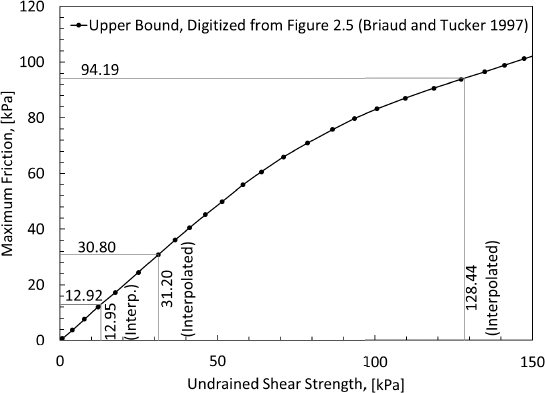
Determine the geotechnical engineering design parameters and establish a profile of the soil deposit. Index parameters (water content, Atterberg limits, unit weight) should be used to help identify the stratigraphy of the soil deposit. The relevant soil data that are needed include soil shear strength and unit weight. An example of the soil stratigraphy for the Briaud and Tucker (1997) Example Problem 1 design example is included as Figure C1. The soil modulus (M) presented in Figure C1 was calculated using Equation 1 based on the Young’s modulus (E) and Poisson’s ratio (ν) values that were provided in Briaud and Tucker (1997). The undrained shear strength values were determined by converting the provided Briaud and Tucker (1997) friction data to undrained shear strength data (Figure C2).
| Eqn. 1 |
Step 2: Determine soil settlement

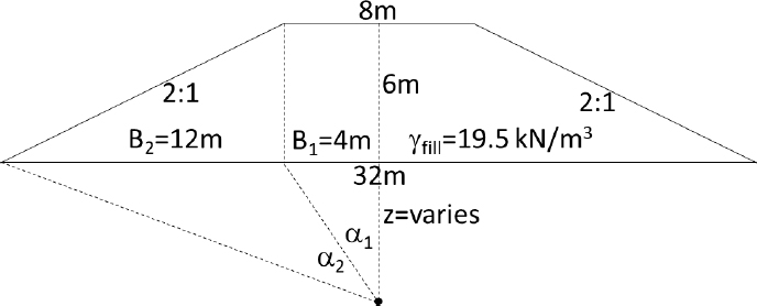
The amount of expected soil settlement is determined using consolidation theory. The settlement profile shown in Figure C3 was created by discretizing the soil into sublayers (50, 0.835m thick layers) and then calculating the amount of settlement within each sublayer resulting from a 6m thick, 8m crest, 32m base embankment fill, with a unit weight of 19.5kN/m3, being placed on top of the two-layer clay soil profile.
A prescribed embankment geometry (6m thick, 8m crest, 32m base) and embankment unit weight (19.5kN/m3) were used to develop the soil settlement profile that is provided in Figure C3. The embankment (width, height, side slope) and unit weight are shown in Figure C4. The settlement profile presented in Figure C3 was developed for points below the center of the embankment using the Osterberg embankment stress distribution, which assumes a symmetric geometry, and provided half of the actual stress influence (Figure C4 and Equations 2 through 4).

| Eqn. 2 |
| Eqn. 3 |
| Eqn. 4 |
For the geometry shown in Figure C4, the embankment is symmetric about the central axis, and the amount of settlement (δ) was determined at different depths along this line of symmetry. Therefore, the influence factor (I), as computed using Equation 2 is multiplied by two (2) to account for both halves of the embankment about the line of symmetry. The increase in stress (∆σ) at each sublayer depth (z) is then determined by multiplying the influence factor with the bearing pressure (q=γfillHfill=117kPa) resulting from the embankment. The α1 and α2 parameters from (Figure C4) along with the Σ(I), ∆σ, and δ values that were calculated for each sublayer are included as Table C3. The consolidation strain (εz) presented in Table C3 was calculated by dividing the change in stress (∆σ) by the constrained modulus (M).
Step 3: Establish pile data
The pile data required to determine the drag load and downdrag include 1) the incremental side resistance acting on the pile(s), 2) the end bearing resistance provided by the pile(s), 3) the unfactored pile head deadload, and 3) the elastic compression of the pile(s). Multiple pile types or pile geometries may be considered to determine the magnitude of downdrag/drag load on the pile(s). To compute the drag load for a given design scenario, the following pile data is required: pile material, pile diameter or pile perimeter, pile cross-sectional area, and pile modulus. The pile considered for this design example was an octagonal pile; the pile diameter was therefore not required. The pile material (pre-stressed concrete), perimeter (1.39m), cross-sectional area (0.145m2), and pile modulus (2.41x10⁷ kN/m2) were considered in this example.
Step 4: Compute incremental side resistance
For a given pile geometry (diameter, length), the incremental side resistance is determined for discretized intervals. Fifty (50) intervals were used to determine the incremental side resistance to compare with the Briaud and Tucker (1997) Example Problem 1 design example. The incremental side resistance was determined by using the total stress analysis “α method” because the undrained shear strength (su) parameters were provided (as determined by the relationship between Briaud and Tucker (1997) maximum friction and undrained shear strength presented previously in Figure C2). Specifically, the procedure and equations (Equations 5 and 6) recommended in Randolph and Murphy (1985) were used. The effective stress (σz0′) used in Equations 5 or 6 was determined using Terzaghi’s effective stress equation with the ground water table assumed to be at the ground surface as shown previously in Figure C1. The effective stress was calculated at the center of each sublayer (as presented in Table C3).
| For : | Eqn. 5 |
| For : | Eqn. 6 |
| with |
Table C3. Calculated settlement parameters.
| Layer Depth [m] | z [m] | Thickness [m] | σzo′ [kPa] | α1 [rad] | α2 [rad] | Σ(I) | ∆σ [kPa] | εz | δ [m] | ||
| 0 | - | 0.8352 | 0.4176 | 0.8352 | 4.0465 | 1.4668 | 0.0779 | 0.9999 | 116.9912 | 0.0040 | 0.0034 |
| 0.8352 | - | 1.6704 | 1.2528 | 0.8352 | 12.1396 | 1.2673 | 0.2254 | 0.9981 | 116.7756 | 0.0040 | 0.0034 |
| 1.6704 | - | 2.5056 | 2.088 | 0.8352 | 20.2327 | 1.0897 | 0.3513 | 0.9919 | 116.0572 | 0.0040 | 0.0033 |
| 2.5056 | - | 3.3408 | 2.9232 | 0.8352 | 28.3258 | 0.9397 | 0.4504 | 0.9805 | 114.7226 | 0.0040 | 0.0033 |
| 3.3408 | - | 4.176 | 3.7584 | 0.8352 | 36.4189 | 0.8165 | 0.5236 | 0.9642 | 112.8139 | 0.0039 | 0.0033 |
| 4.176 | - | 5.0112 | 4.5936 | 0.8352 | 44.5120 | 0.7164 | 0.5748 | 0.9440 | 110.4464 | 0.0038 | 0.0032 |
| 5.0112 | - | 5.8464 | 5.4288 | 0.8352 | 52.6051 | 0.6350 | 0.6087 | 0.9209 | 107.7477 | 0.0037 | 0.0031 |
| 5.8464 | - | 6.6816 | 6.264 | 0.8352 | 60.6982 | 0.5683 | 0.6293 | 0.8960 | 104.8309 | 0.0036 | 0.0030 |
| 6.6816 | - | 7.5168 | 7.0992 | 0.8352 | 68.7912 | 0.5131 | 0.6401 | 0.8700 | 101.7873 | 0.0035 | 0.0029 |
| 7.5168 | - | 8.352 | 7.9344 | 0.8352 | 76.8843 | 0.4669 | 0.6435 | 0.8435 | 98.6867 | 0.0034 | 0.0028 |
| 8.352 | - | 9.1872 | 8.7696 | 0.8352 | 84.9774 | 0.4279 | 0.6415 | 0.8169 | 95.5815 | 0.0033 | 0.0028 |
| 9.1872 | - | 10.0224 | 9.6048 | 0.8352 | 93.0705 | 0.3946 | 0.6355 | 0.7907 | 92.5100 | 0.0032 | 0.0027 |
| 10.0224 | - | 10.8576 | 10.44 | 0.8352 | 101.1636 | 0.3659 | 0.6268 | 0.7650 | 89.4999 | 0.0031 | 0.0026 |
| 10.8576 | - | 11.6928 | 11.2752 | 0.8352 | 109.2567 | 0.3409 | 0.6160 | 0.7399 | 86.5704 | 0.0030 | 0.0025 |
| 11.6928 | - | 12.528 | 12.1104 | 0.8352 | 117.3498 | 0.3190 | 0.6039 | 0.7157 | 83.7345 | 0.0029 | 0.0024 |
| 12.528 | - | 13.3632 | 12.9456 | 0.8352 | 125.4429 | 0.2997 | 0.5909 | 0.6923 | 81.0005 | 0.0028 | 0.0023 |
| 13.3632 | - | 14.1984 | 13.7808 | 0.8352 | 133.5360 | 0.2825 | 0.5773 | 0.6699 | 78.3730 | 0.0027 | 0.0023 |
| 14.1984 | - | 15.0336 | 14.616 | 0.8352 | 141.6290 | 0.2671 | 0.5634 | 0.6483 | 75.8540 | 0.0026 | 0.0022 |
| 15.0336 | - | 15.8688 | 15.4512 | 0.8352 | 149.7221 | 0.2533 | 0.5495 | 0.6277 | 73.4433 | 0.0025 | 0.0021 |
| 15.8688 | - | 16.704 | 16.2864 | 0.8352 | 157.8152 | 0.2408 | 0.5357 | 0.6080 | 71.1395 | 0.0025 | 0.0021 |
| 16.704 | - | 17.5392 | 17.1216 | 0.8352 | 165.9083 | 0.2295 | 0.5220 | 0.5892 | 68.9400 | 0.0024 | 0.0020 |
| 17.5392 | - | 18.3744 | 17.9568 | 0.8352 | 174.0014 | 0.2192 | 0.5087 | 0.5713 | 66.8415 | 0.0023 | 0.0019 |
| 18.3744 | - | 19.2096 | 18.792 | 0.8352 | 182.0945 | 0.2097 | 0.4956 | 0.5542 | 64.8402 | 0.0022 | 0.0019 |
| 19.2096 | - | 20.0448 | 19.6272 | 0.8352 | 190.1876 | 0.2010 | 0.4829 | 0.5379 | 62.9321 | 0.0022 | 0.0018 |
| 20.0448 | - | 20.88 | 20.4624 | 0.8352 | 198.2807 | 0.1930 | 0.4706 | 0.5223 | 61.1129 | 0.0021 | 0.0018 |
| 20.88 | - | 21.7152 | 21.2976 | 0.8352 | 206.3737 | 0.1857 | 0.4587 | 0.5075 | 59.3784 | 0.0020 | 0.0017 |
| 21.7152 | - | 22.5504 | 22.1328 | 0.8352 | 214.4668 | 0.1788 | 0.4471 | 0.4934 | 57.7242 | 0.0020 | 0.0017 |
| 22.5504 | - | 23.3856 | 22.968 | 0.8352 | 222.5599 | 0.1724 | 0.4360 | 0.4799 | 56.1463 | 0.0019 | 0.0016 |
| 23.3856 | - | 24.2208 | 23.8032 | 0.8352 | 230.6530 | 0.1665 | 0.4253 | 0.4670 | 54.6405 | 0.0019 | 0.0016 |
| 24.2208 | - | 25.056 | 24.6384 | 0.8352 | 238.7461 | 0.1609 | 0.4150 | 0.4547 | 53.2030 | 0.0018 | 0.0015 |
| 25.056 | - | 25.8912 | 25.4736 | 0.8352 | 246.8392 | 0.1558 | 0.4051 | 0.4430 | 51.8301 | 0.0018 | 0.0015 |
| 25.8912 | - | 26.7264 | 26.3088 | 0.8352 | 254.9323 | 0.1509 | 0.3955 | 0.4318 | 50.5182 | 0.0017 | 0.0015 |
| 26.7264 | - | 27.5616 | 27.144 | 0.8352 | 263.0254 | 0.1463 | 0.3863 | 0.4211 | 49.2638 | 0.0017 | 0.0014 |
| 27.5616 | - | 28.3968 | 27.9792 | 0.8352 | 271.1184 | 0.1420 | 0.3775 | 0.4108 | 48.0640 | 0.0017 | 0.0014 |
| 28.3968 | - | 29.232 | 28.8144 | 0.8352 | 279.2115 | 0.1379 | 0.3689 | 0.4010 | 46.9155 | 0.0016 | 0.0014 |
| 29.232 | - | 30.0672 | 29.6496 | 0.8352 | 287.3046 | 0.1341 | 0.3608 | 0.3916 | 45.8156 | 0.0016 | 0.0013 |
| 30.0672 | - | 30.9024 | 30.4848 | 0.8352 | 295.3977 | 0.1305 | 0.3529 | 0.3826 | 44.7616 | 0.0015 | 0.0013 |
| 30.9024 | - | 31.7376 | 31.32 | 0.8352 | 303.4908 | 0.1270 | 0.3453 | 0.3739 | 43.7510 | 0.0015 | 0.0013 |
| 31.7376 | - | 32.5728 | 32.1552 | 0.8352 | 311.5839 | 0.1238 | 0.3380 | 0.3657 | 42.7814 | 0.0015 | 0.0012 |
| 32.5728 | - | 33.408 | 32.9904 | 0.8352 | 319.6770 | 0.1207 | 0.3309 | 0.3577 | 41.8506 | 0.0014 | 0.0012 |
| 33.408 | - | 34.2432 | 33.8256 | 0.8352 | 327.7701 | 0.1177 | 0.3241 | 0.3501 | 40.9566 | 0.0014 | 0.0012 |
| 34.2432 | - | 35.0784 | 34.6608 | 0.8352 | 335.8632 | 0.1149 | 0.3176 | 0.3427 | 40.0973 | 0.0014 | 0.0012 |
| 35.0784 | - | 35.9136 | 35.496 | 0.8352 | 343.9562 | 0.1122 | 0.3113 | 0.3356 | 39.2710 | 0.0014 | 0.0011 |
| 35.9136 | - | 36.7488 | 36.3312 | 0.8352 | 352.0493 | 0.1097 | 0.3052 | 0.3289 | 38.4759 | 0.0013 | 0.0011 |
| 36.7488 | - | 37.584 | 37.1664 | 0.8352 | 360.1424 | 0.1072 | 0.2993 | 0.3223 | 37.7104 | 0.0013 | 0.0011 |
| 37.584 | - | 38.4192 | 38.0016 | 0.8352 | 368.2355 | 0.1049 | 0.2936 | 0.3160 | 36.9730 | 0.0013 | 0.0011 |
| 38.4192 | - | 39.2544 | 38.8368 | 0.8352 | 376.3286 | 0.1026 | 0.2882 | 0.3099 | 36.2624 | 0.0013 | 0.0010 |
| 39.2544 | - | 40.0896 | 39.672 | 0.8352 | 384.4217 | 0.1005 | 0.2829 | 0.3041 | 35.5770 | 0.0012 | 0.0010 |
| 40.0896 | - | 40.9248 | 40.5072 | 0.8352 | 392.5148 | 0.0984 | 0.2778 | 0.2984 | 34.9158 | 0.0012 | 0.0010 |
| 40.9248 | - | 41.76 | 41.3424 | 0.8352 | 400.6079 | 0.0965 | 0.2728 | 0.2930 | 34.2774 | 0.0012 | 0.0010 |
| z = layer midpoint depth, |
|||||||||||
The nominal unit side resistance (fn) for each sublayer was calculated by multiplying the α factor by the undrained shear strength using Equation 7. Likewise, the side resistance (Fs) for each sublayer was determined by multiplying the nominal side resistance by the area of the pile in contact with the soil within the given sublayer (Equation 8). The total side resistance for the pile was determined by summing the side resistance from each sublayer.
| Eqn. 7 |
| Eqn. 8 |
The values that were calculated for the pile and soil properties presented in or inferred from the Briaud and Tucker (1997) Example Problem 1 design example are included in Table C4. These values include the vertical effective stress (σvo′), undrained shear strength (su), alpha value (α), nominal side resistance (fn), and side resistance (Fs) obtained for each sublayer.
Step 5: Develop a depth-dependent load profile
The depth-varying load profile is developed by determining the cumulative load in the pile, as a function of depth. Beginning at the top of the pile, the cumulative load in the pile is determined by adding the discretized side resistance for a given sublayer to the previous cumulative total. For this example, immediately after driving, the load in the pile at each depth was equal to the cumulative side resistance value at that depth prior to application of the top load on the pile. Assuming the top load transferred to the toe of the pile, the unfactored amount of top load that was added to the pile top was also added to the cumulative load in the pile value for all depths. Therefore, at a depth of 0m, the load in the pile was equal to the unfactored top load applied to the pile. At the bottom of the first increment, the cumulative side resistance was the combination of the unfactored top load and the incremental side resistance developed over the length of the first increment. The calculated load profile, within the octagonal precast concrete pile that was described in the Briaud and Tucker (1997) Example Problem 1 design example, is shown in Figure C5. Specifically, the data for the load profile after driving and the load profile after top load application are presented as Figures C5a and C5b, respectively. The tabulated data are also presented in Table C5.
Table C4. Calculated pile side resistance parameters.
| Layer Depth | z | Thickness | σzo′ | su | α | fn | Fs | ||
| [m] | [m] | [m] | [kPa] | [kPa] | [kPa] | [kN] | |||
| 0 | - | 0.8352 | 0.4176 | 0.8352 | 4.0465 | 13.29 | 0.35 | 0.00 | 0.00 |
| 0.8352 | - | 1.6704 | 1.2528 | 0.8352 | 12.1396 | 13.95 | 0.45 | 6.32 | 7.34 |
| 1.6704 | - | 2.5056 | 2.088 | 0.8352 | 20.2327 | 14.62 | 0.55 | 8.07 | 9.37 |
| 2.5056 | - | 3.3408 | 2.9232 | 0.8352 | 28.3258 | 15.29 | 0.64 | 9.76 | 11.33 |
| 3.3408 | - | 4.176 | 3.7584 | 0.8352 | 36.4189 | 15.95 | 0.71 | 11.31 | 13.13 |
| 4.176 | - | 5.0112 | 4.5936 | 0.8352 | 44.5120 | 16.62 | 0.77 | 12.76 | 14.81 |
| 5.0112 | - | 5.8464 | 5.4288 | 0.8352 | 52.6051 | 17.29 | 0.82 | 14.14 | 16.42 |
| 5.8464 | - | 6.6816 | 6.264 | 0.8352 | 60.6982 | 17.95 | 0.86 | 15.48 | 17.98 |
| 6.6816 | - | 7.5168 | 7.0992 | 0.8352 | 68.7912 | 18.62 | 0.90 | 16.79 | 19.49 |
| 7.5168 | - | 8.352 | 7.9344 | 0.8352 | 76.8843 | 19.29 | 0.94 | 18.06 | 20.97 |
| 8.352 | - | 9.1872 | 8.7696 | 0.8352 | 84.9774 | 19.95 | 0.97 | 19.31 | 22.42 |
| 9.1872 | - | 10.0224 | 9.6048 | 0.8352 | 93.0705 | 20.62 | 1.00 | 20.55 | 23.86 |
| 10.0224 | - | 10.8576 | 10.44 | 0.8352 | 101.1636 | 21.29 | 1.02 | 21.77 | 25.27 |
| 10.8576 | - | 11.6928 | 11.2752 | 0.8352 | 109.2567 | 21.95 | 1.05 | 22.97 | 26.67 |
| 11.6928 | - | 12.528 | 12.1104 | 0.8352 | 117.3498 | 22.62 | 1.07 | 24.17 | 28.06 |
| 12.528 | - | 13.3632 | 12.9456 | 0.8352 | 125.4429 | 23.29 | 1.09 | 25.35 | 29.43 |
| 13.3632 | - | 14.1984 | 13.7808 | 0.8352 | 133.5360 | 23.95 | 1.11 | 26.53 | 30.80 |
| 14.1984 | - | 15.0336 | 14.616 | 0.8352 | 141.6290 | 24.62 | 1.12 | 27.70 | 32.16 |
| 15.0336 | - | 15.8688 | 15.4512 | 0.8352 | 149.7221 | 25.29 | 1.14 | 28.86 | 33.51 |
| 15.8688 | - | 16.704 | 16.2864 | 0.8352 | 157.8152 | 25.95 | 1.16 | 30.02 | 34.85 |
| 16.704 | - | 17.5392 | 17.1216 | 0.8352 | 165.9083 | 26.62 | 1.17 | 31.17 | 36.19 |
| 17.5392 | - | 18.3744 | 17.9568 | 0.8352 | 174.0014 | 27.29 | 1.18 | 32.32 | 37.52 |
| 18.3744 | - | 19.2096 | 18.792 | 0.8352 | 182.0945 | 27.95 | 1.20 | 33.46 | 38.85 |
| 19.2096 | - | 20.0448 | 19.6272 | 0.8352 | 190.1876 | 28.62 | 1.21 | 34.61 | 40.17 |
| 20.0448 | - | 20.88 | 20.4624 | 0.8352 | 198.2807 | 29.29 | 1.22 | 35.74 | 41.50 |
| 20.88 | - | 21.7152 | 21.2976 | 0.8352 | 206.3737 | 29.95 | 1.23 | 36.88 | 42.81 |
| 21.7152 | - | 22.5504 | 22.1328 | 0.8352 | 214.4668 | 30.62 | 1.24 | 38.01 | 44.13 |
| 22.5504 | - | 23.3856 | 22.968 | 0.8352 | 222.5599 | 31.76 | 1.24 | 39.43 | 45.78 |
| 23.3856 | - | 24.2208 | 23.8032 | 0.8352 | 230.6530 | 36.05 | 1.19 | 42.77 | 49.66 |
| 24.2208 | - | 25.056 | 24.6384 | 0.8352 | 238.7461 | 40.35 | 1.14 | 46.04 | 53.45 |
| 25.056 | - | 25.8912 | 25.4736 | 0.8352 | 246.8392 | 44.65 | 1.10 | 49.24 | 57.16 |
| 25.8912 | - | 26.7264 | 26.3088 | 0.8352 | 254.9323 | 48.94 | 1.07 | 52.39 | 60.82 |
| 26.7264 | - | 27.5616 | 27.144 | 0.8352 | 263.0254 | 53.24 | 1.04 | 55.51 | 64.44 |
| 27.5616 | - | 28.3968 | 27.9792 | 0.8352 | 271.1184 | 57.54 | 1.02 | 58.58 | 68.01 |
| 28.3968 | - | 29.232 | 28.8144 | 0.8352 | 279.2115 | 61.84 | 1.00 | 61.63 | 71.55 |
| 29.232 | - | 30.0672 | 29.6496 | 0.8352 | 287.3046 | 66.13 | 0.98 | 64.65 | 75.06 |
| 30.0672 | - | 30.9024 | 30.4848 | 0.8352 | 295.3977 | 70.43 | 0.96 | 67.65 | 78.54 |
| 30.9024 | - | 31.7376 | 31.32 | 0.8352 | 303.4908 | 74.73 | 0.95 | 70.63 | 82.00 |
| 31.7376 | - | 32.5728 | 32.1552 | 0.8352 | 311.5839 | 79.02 | 0.93 | 73.60 | 85.44 |
| 32.5728 | - | 33.408 | 32.9904 | 0.8352 | 319.6770 | 83.32 | 0.92 | 76.55 | 88.87 |
| 33.408 | - | 34.2432 | 33.8256 | 0.8352 | 327.7701 | 87.62 | 0.91 | 79.49 | 92.28 |
| 34.2432 | - | 35.0784 | 34.6608 | 0.8352 | 335.8632 | 91.91 | 0.90 | 82.41 | 95.67 |
| 35.0784 | - | 35.9136 | 35.496 | 0.8352 | 343.9562 | 96.21 | 0.89 | 85.32 | 99.06 |
| 35.9136 | - | 36.7488 | 36.3312 | 0.8352 | 352.0493 | 100.51 | 0.88 | 88.23 | 102.43 |
| 36.7488 | - | 37.584 | 37.1664 | 0.8352 | 360.1424 | 104.80 | 0.87 | 91.12 | 105.79 |
| 37.584 | - | 38.4192 | 38.0016 | 0.8352 | 368.2355 | 109.10 | 0.86 | 94.01 | 109.14 |
| 38.4192 | - | 39.2544 | 38.8368 | 0.8352 | 376.3286 | 113.40 | 0.85 | 96.89 | 112.49 |
| 39.2544 | - | 40.0896 | 39.672 | 0.8352 | 384.4217 | 117.69 | 0.85 | 99.77 | 115.82 |
| 40.0896 | - | 40.9248 | 40.5072 | 0.8352 | 392.5148 | 121.99 | 0.84 | 102.64 | 119.15 |
| 40.9248 | - | 41.76 | 41.3424 | 0.8352 | 400.6079 | 126.29 | 0.84 | 105.50 | 122.48 |
| z = layer midpoint depth, σzo′ = vertical effective stress, su = undrained shear strength, α = total stress side resistance value, fn=nominal unit side resistance, Fs=sublayer side resistance. Note: fn neglected for top 1.5m | |||||||||

Table C5. Calculated load as a function of depth.
| Layer Depth | z | QAD | QwUTL | ||
| [m] | [m] | [kN] | [kN] | ||
| 0 | - | 0.8352 | 0.4176 | 0.00 | 2225.00 |
| 0.8352 | - | 1.6704 | 1.2528 | 7.34 | 2232.34 |
| 1.6704 | - | 2.5056 | 2.088 | 16.70 | 2241.70 |
| 2.5056 | - | 3.3408 | 2.9232 | 28.04 | 2253.04 |
| 3.3408 | - | 4.176 | 3.7584 | 41.16 | 2266.16 |
| 4.176 | - | 5.0112 | 4.5936 | 55.97 | 2280.97 |
| 5.0112 | - | 5.8464 | 5.4288 | 72.39 | 2297.39 |
| 5.8464 | - | 6.6816 | 6.264 | 90.37 | 2315.37 |
| 6.6816 | - | 7.5168 | 7.0992 | 109.86 | 2334.86 |
| 7.5168 | - | 8.352 | 7.9344 | 130.83 | 2355.83 |
| 8.352 | - | 9.1872 | 8.7696 | 153.25 | 2378.25 |
| 9.1872 | - | 10.0224 | 9.6048 | 177.11 | 2402.11 |
| 10.0224 | - | 10.8576 | 10.44 | 202.38 | 2427.38 |
| 10.8576 | - | 11.6928 | 11.2752 | 229.04 | 2454.04 |
| 11.6928 | - | 12.528 | 12.1104 | 257.10 | 2482.10 |
| 12.528 | - | 13.3632 | 12.9456 | 286.53 | 2511.53 |
| 13.3632 | - | 14.1984 | 13.7808 | 317.33 | 2542.33 |
| 14.1984 | - | 15.0336 | 14.616 | 349.48 | 2574.48 |
| 15.0336 | - | 15.8688 | 15.4512 | 382.99 | 2607.99 |
| 15.8688 | - | 16.704 | 16.2864 | 417.84 | 2642.84 |
| 16.704 | - | 17.5392 | 17.1216 | 454.03 | 2679.03 |
| 17.5392 | - | 18.3744 | 17.9568 | 491.55 | 2716.55 |
| 18.3744 | - | 19.2096 | 18.792 | 530.40 | 2755.40 |
| 19.2096 | - | 20.0448 | 19.6272 | 570.57 | 2795.57 |
| 20.0448 | - | 20.88 | 20.4624 | 612.07 | 2837.07 |
| 20.88 | - | 21.7152 | 21.2976 | 654.88 | 2879.88 |
| 21.7152 | - | 22.5504 | 22.1328 | 699.01 | 2924.01 |
| 22.5504 | - | 23.3856 | 22.968 | 744.79 | 2969.79 |
| 23.3856 | - | 24.2208 | 23.8032 | 794.44 | 3019.44 |
| 24.2208 | - | 25.056 | 24.6384 | 847.89 | 3072.89 |
| 25.056 | - | 25.8912 | 25.4736 | 905.05 | 3130.05 |
| 25.8912 | - | 26.7264 | 26.3088 | 965.88 | 3190.88 |
| 26.7264 | - | 27.5616 | 27.144 | 1030.32 | 3255.32 |
| 27.5616 | - | 28.3968 | 27.9792 | 1098.33 | 3323.33 |
| 28.3968 | - | 29.232 | 28.8144 | 1169.88 | 3394.88 |
| 29.232 | - | 30.0672 | 29.6496 | 1244.93 | 3469.93 |
| 30.0672 | - | 30.9024 | 30.4848 | 1323.47 | 3548.47 |
| 30.9024 | - | 31.7376 | 31.32 | 1405.48 | 3630.48 |
| 31.7376 | - | 32.5728 | 32.1552 | 1490.92 | 3715.92 |
| 32.5728 | - | 33.408 | 32.9904 | 1579.79 | 3804.79 |
| 33.408 | - | 34.2432 | 33.8256 | 1672.06 | 3897.06 |
| 34.2432 | - | 35.0784 | 34.6608 | 1767.74 | 3992.74 |
| 35.0784 | - | 35.9136 | 35.496 | 1866.79 | 4091.79 |
| 35.9136 | - | 36.7488 | 36.3312 | 1969.22 | 4194.22 |
| 36.7488 | - | 37.584 | 37.1664 | 2075.01 | 4300.01 |
| 37.584 | - | 38.4192 | 38.0016 | 2184.15 | 4409.15 |
| 38.4192 | - | 39.2544 | 38.8368 | 2296.64 | 4521.64 |
| 39.2544 | - | 40.0896 | 39.672 | 2412.46 | 4637.46 |
| 40.0896 | - | 40.9248 | 40.5072 | 2531.61 | 4756.61 |
| 40.9248 | - | 41.76 | 41.3424 | 2654.09 | 4879.09 |
| QAD= load in pile after driving, QwUTL= load in pile with addition of unfactored top load |
|||||
Step 6: Calculate end bearing resistance and develop the depth-dependent resistance profile
The depth-dependent resistance profile is determined in a similar fashion to the development of the load profile graph. The resistance profile accumulates the resistance from the bottom of the pile to the top of the pile and includes the end bearing resistance. For the clay profile that was investigated, the end bearing resistance (Rt) was calculated using the undrained shear strength at the toe of the pile (su) and the cross-sectional area at the end of the pile (At) as obtained from Equations 9 and 10.
| Eqn. 9 |
| Eqn. 10 |
The calculated resistance profile, within the octagonal precast concrete pile that was described in the Briaud and Tucker (1997) Example Problem 1 design example, is shown in Figure C6. Unlike the load profile, the resistance profile does not change in the presence of the unfactored top load. The tabulated data are also presented in Table C6.

Step 7: Develop the depth-dependent combined load profile for the pile
The combined load and resistance profile graph for the pile analyzed for the example presented herein is presented in Figure C7. The combined load plot begins at the top of the pile and follows the load curve until the intersection with the resistance curve then follows the resistance curve until the toe of the pile is reached. The combined profile includes the application of the unfactored top load on the pile and the end bearing resistance at the toe of the pile.
Table C6. Calculated resistance as a function of depth.
| Layer Depth | z | R | R= resistance from soil surrounding pile; resistance values are calculated at the top of each sublayer; the bottom sublayer includes the summation of the end bearing resistance and the side resistance in the bottom sublayer. | ||
| [m] | [m] | [kN] | |||
| 0 | - | 0.8352 | 0.4176 | 2821.70 | |
| 0.8352 | - | 1.6704 | 1.2528 | 2821.70 | |
| 1.6704 | - | 2.5056 | 2.088 | 2814.36 | |
| 2.5056 | - | 3.3408 | 2.9232 | 2805.00 | |
| 3.3408 | - | 4.176 | 3.7584 | 2793.66 | |
| 4.176 | - | 5.0112 | 4.5936 | 2780.54 | |
| 5.0112 | - | 5.8464 | 5.4288 | 2765.73 | |
| 5.8464 | - | 6.6816 | 6.264 | 2749.31 | |
| 6.6816 | - | 7.5168 | 7.0992 | 2731.33 | |
| 7.5168 | - | 8.352 | 7.9344 | 2711.84 | |
| 8.352 | - | 9.1872 | 8.7696 | 2690.87 | |
| 9.1872 | - | 10.0224 | 9.6048 | 2668.45 | |
| 10.0224 | - | 10.8576 | 10.44 | 2644.59 | |
| 10.8576 | - | 11.6928 | 11.2752 | 2619.32 | |
| 11.6928 | - | 12.528 | 12.1104 | 2592.65 | |
| 12.528 | - | 13.3632 | 12.9456 | 2564.60 | |
| 13.3632 | - | 14.1984 | 13.7808 | 2535.17 | |
| 14.1984 | - | 15.0336 | 14.616 | 2504.37 | |
| 15.0336 | - | 15.8688 | 15.4512 | 2472.22 | |
| 15.8688 | - | 16.704 | 16.2864 | 2438.71 | |
| 16.704 | - | 17.5392 | 17.1216 | 2403.86 | |
| 17.5392 | - | 18.3744 | 17.9568 | 2367.67 | |
| 18.3744 | - | 19.2096 | 18.792 | 2330.15 | |
| 19.2096 | - | 20.0448 | 19.6272 | 2291.30 | |
| 20.0448 | - | 20.88 | 20.4624 | 2251.13 | |
| 20.88 | - | 21.7152 | 21.2976 | 2209.63 | |
| 21.7152 | - | 22.5504 | 22.1328 | 2166.82 | |
| 22.5504 | - | 23.3856 | 22.968 | 2122.69 | |
| 23.3856 | - | 24.2208 | 23.8032 | 2076.91 | |
| 24.2208 | - | 25.056 | 24.6384 | 2027.26 | |
| 25.056 | - | 25.8912 | 25.4736 | 1973.81 | |
| 25.8912 | - | 26.7264 | 26.3088 | 1916.65 | |
| 26.7264 | - | 27.5616 | 27.144 | 1855.82 | |
| 27.5616 | - | 28.3968 | 27.9792 | 1791.38 | |
| 28.3968 | - | 29.232 | 28.8144 | 1723.37 | |
| 29.232 | - | 30.0672 | 29.6496 | 1651.82 | |
| 30.0672 | - | 30.9024 | 30.4848 | 1576.77 | |
| 30.9024 | - | 31.7376 | 31.32 | 1498.23 | |
| 31.7376 | - | 32.5728 | 32.1552 | 1416.22 | |
| 32.5728 | - | 33.408 | 32.9904 | 1330.78 | |
| 33.408 | - | 34.2432 | 33.8256 | 1241.91 | |
| 34.2432 | - | 35.0784 | 34.6608 | 1149.64 | |
| 35.0784 | - | 35.9136 | 35.496 | 1053.96 | |
| 35.9136 | - | 36.7488 | 36.3312 | 954.91 | |
| 36.7488 | - | 37.584 | 37.1664 | 852.48 | |
| 37.584 | - | 38.4192 | 38.0016 | 746.69 | |
| 38.4192 | - | 39.2544 | 38.8368 | 637.55 | |
| 39.2544 | - | 40.0896 | 39.672 | 525.06 | |
| 40.0896 | - | 40.9248 | 40.5072 | 409.24 | |
| 40.9248 | - | 41.76 | 41.3424 | 290.09 | |
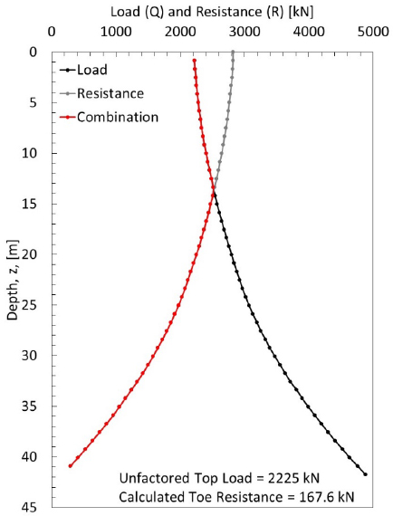
Step 8: Identify the location of the neutral plane from the combined load and resistance curve
The neutral plane is located at the intersection of the load and resistance curves when plotted on the same graph. The neutral plane is located at 13.36m based on the calculations that were performed (Figure C8). The amount of load in the pile at the location of the neutral plane (2511kN) is similar to the 2535kN of load predicted by Briaud and Tucker (1997). The calculated depth of the neutral plane (13.36m) was deeper than the 12.53m neutral plane location computed by Briaud and Tucker (1997).
Step 9: Calculate the amount of drag load in the pile
The amount of drag load in the pile is equal to the amount of load in the pile at the location of the neutral plane minus the amount of unfactored load applied to the top of pile. Based on the calculations, the drag load was determined to be 286kN. Briaud and Tucker (1997) calculated the amount of drag load to be 310kN. Specifically, the drag load for the octagonal precast concrete pile is shown in Figure C9.


Step 10: Calculate the toe settlement and elastic compression in the pile
The elastic compression (δEC) for each segment of the pile is calculated using the load within the pile (load [Q] above the neutral plane and resistance [R] below the neutral plane, from Figure C9 shown previously), the cross-sectional area of the pile (A), the elastic modulus of the pile (E), and the segmental length of the pile (Ls). Specifically, the elastic compression for each segment (δEC,s) of the pile is determined using Equation 11. The cumulative elastic compression in the pile is then determined by accumulating each of the elastic compression values from the bottom of the pile to the top of the pile (Equation 12). The calculated segmental and cumulative elastic compression values are shown in Figure C10 and tabulated in Table C7. The toe movement is combined with the geotechnical resistance in Step 11.
| Eqn. 11 |
| Eqn. 12 |
Step 11: Calculate the geotechnical resistance of the pile
The nominal compression resistance of the pile is determined using the Davisson Method (Davisson, 1972). Typically, the Davisson Method is intended to be used to determine the nominal axial downward resistance based on a measured load-displacement curve from a full-scale load test performed on a pile. A simulated load-displacement curve is suggested herein to enable estimation of the location of the neutral plane based on estimated pile and soil settlement data prior to commencement of fieldwork or full-scale testing. The suggested load-displacement curve is developed using the DeCock (2009) method based on Chin’s Hyperbolic Model. Specifically, the end resistance (Rt) and side resistance (Rs) values are computed using Equations 13 and 14 for prescribed levels of toe displacement (δt) and side displacement (δs). A flexibility factor (Kt or Ks) is included in each equation to account for the initial slope of the Rt/Rtu-δt curve and the f/fn-δs curve, respectively. The respective flexibility factors are calculated using Equations 15 and 16. The end bearing resistance flexibility factor is a function of the pile diameter and the secant modulus at 25 percent of the shear strength of the soil (E25,s) at the toe of the pile. As described in DeCock (2009), the secant modulus at 25 percent of the shear strength (E25,s), in units of [kPa], is calculated as being 1000 times the undrained shear strength for stiff soils. The dimensionless parameter Ms is typically 0.001 for stiff soils. As shown previously in Figure C1, an undrained shear strength of 128 kPa was used for this example. Likewise, the diameter of the octagonal pile (D) was assumed to be the distance across the octagonal pile (419mm), as reported on Page 85 of Briaud and Tucker (1997).
The disparity between the amount of movement required to mobilize the side resistance and the amount of movement required to mobilize the end bearing resistance is known but not considered for this example. To simplify calculations, rigid body movement of the pile is assumed to fully mobilize the pile in both side resistance and end bearing. Thereby, the movement of the top of the pile and the toe of the pile are equal. Displacement intervals of 0.0005m were investigated for movements of 0.00m to 0.01m and intervals of 0.005m were investigated between 0.01m and 0.05m. The asymptotic ultimate value of load that was observed at very large displacements was assumed to develop at a displacement value of 10 percent of the pile diameter (Equation 17).

Table C7. Calculated elastic compression in the pile as a function of depth.
| z | δEC,s | δEC | Comments: z=depth, Q=load, R=resistance, δEC,s=segmental elastic compression, δEC=cumulative elastic compression (from bottom to top), A=pile cross-sectional area=0.145[m2] Ep=pile elastic modulus=2.41E+07[kPa] Ls=length of each pile segment=0.8532[m] |
|
| [m] | [kN] | [m] | [m] | |
| 0.4176 | 2225.00 | 0.0005 | 0.0225 | |
| 1.2528 | 2232.34 | 0.0005 | 0.0220 | |
| 2.088 | 2241.70 | 0.0005 | 0.0215 | |
| 2.9232 | 2253.04 | 0.0005 | 0.0209 | |
| 3.7584 | 2266.16 | 0.0005 | 0.0204 | |
| 4.5936 | 2280.97 | 0.0005 | 0.0198 | |
| 5.4288 | 2297.39 | 0.0005 | 0.0193 | |
| 6.264 | 2315.37 | 0.0006 | 0.0188 | |
| 7.0992 | 2334.86 | 0.0006 | 0.0182 | |
| 7.9344 | 2355.83 | 0.0006 | 0.0176 | |
| 8.7696 | 2378.25 | 0.0006 | 0.0171 | |
| 9.6048 | 2402.11 | 0.0006 | 0.0165 | |
| 10.44 | 2427.38 | 0.0006 | 0.0159 | |
| 11.2752 | 2454.04 | 0.0006 | 0.0154 | |
| 12.1104 | 2482.10 | 0.0006 | 0.0148 | |
| 12.9456 | 2511.53 | 0.0006 | 0.0142 | |
| 13.7808 | 2535.17 | 0.0006 | 0.0136 | |
| 14.616 | 2504.37 | 0.0006 | 0.0130 | |
| 15.4512 | 2472.22 | 0.0006 | 0.0124 | |
| 16.2864 | 2438.71 | 0.0006 | 0.0118 | |
| 17.1216 | 2403.86 | 0.0006 | 0.0112 | |
| 17.9568 | 2367.67 | 0.0006 | 0.0106 | |
| 18.792 | 2330.15 | 0.0006 | 0.0101 | |
| 19.6272 | 2291.30 | 0.0005 | 0.0095 | |
| 20.4624 | 2251.13 | 0.0005 | 0.0090 | |
| 21.2976 | 2209.63 | 0.0005 | 0.0084 | |
| 22.1328 | 2166.82 | 0.0005 | 0.0079 | |
| 22.968 | 2122.69 | 0.0005 | 0.0074 | |
| 23.8032 | 2076.91 | 0.0005 | 0.0069 | |
| 24.6384 | 2027.26 | 0.0005 | 0.0064 | |
| 25.4736 | 1973.81 | 0.0005 | 0.0059 | |
| 26.3088 | 1916.65 | 0.0005 | 0.0054 | |
| 27.144 | 1855.82 | 0.0004 | 0.0049 | |
| 27.9792 | 1791.38 | 0.0004 | 0.0045 | |
| 28.8144 | 1723.37 | 0.0004 | 0.0041 | |
| 29.6496 | 1651.82 | 0.0004 | 0.0037 | |
| 30.4848 | 1576.77 | 0.0004 | 0.0033 | |
| 31.32 | 1498.23 | 0.0004 | 0.0029 | |
| 32.1552 | 1416.22 | 0.0003 | 0.0025 | |
| 32.9904 | 1330.78 | 0.0003 | 0.0022 | |
| 33.8256 | 1241.91 | 0.0003 | 0.0019 | |
| 34.6608 | 1149.64 | 0.0003 | 0.0016 | |
| 35.496 | 1053.96 | 0.0003 | 0.0013 | |
| 36.3312 | 954.91 | 0.0002 | 0.0011 | |
| 37.1664 | 852.48 | 0.0002 | 0.0008 | |
| 38.0016 | 746.69 | 0.0002 | 0.0006 | |
| 38.8368 | 637.55 | 0.0002 | 0.0004 | |
| 39.672 | 525.06 | 0.0001 | 0.0003 | |
| 40.5072 | 409.24 | 0.0001 | 0.0002 | |
| 41.3424 | 290.09 | 0.0001 | 0.0001 |
An ultimate value (Rtu) that is larger than the nominal net end bearing (Rt,10%; defined as R in Equation 10 that was previously presented) is used because the ultimate limit state Rt,10% value is typically defined at a movement of 10 percent of the pile diameter which may not correspond with the service limit state. The tabulated movement and the corresponding side resistance, end bearing resistance, and total resistance are included in Table C8.
| Eqn. 13 |
| Eqn. 14 |
| Eqn. 15 |
| Eqn. 16 |
| Eqn. 17 |
The predicted load-displacement curve for the pile is presented in Figure C11. This total resistance curve includes the influence from side resistance and end resistance. Also presented in Figure C11 is the Davisson Method line that was used to determine the nominal axial geotechnical resistance (2800kN) and displacement (0.041m) at failure for the pile that was analyzed.
This pile was not tipped into rock. Therefore, the location and settlement of the neutral plane can be determined in Step 12. Moreover, the location of the neutral plane determined from the combined load-resistance curve in Step 8 can then be compared with the location of the neutral plane determined from the soil settlement-pile settlement curve that will be determined in Step 12.
Step 12: Identify the location of and settlement at the neutral plane (from the soil settlement-pile settlement curve)
When using the soil settlement-pile settlement graph, the neutral plane is located at the intersection of the soil settlement and pile settlement curves when plotted on the same graph as a function of depth. The pile settlement is obtained by adding the settlement (0.041m) that was reported in Figure C11 with the elastic compression as a function of depth that was previously reported in Figure C10. These values are tabulated as Table C9. As shown in Figure C12, the neutral plane is located at a depth of 12.1m based on the calculations that were performed in Step 12. Moreover, the downdrag was determined to be 0.055m.
When comparing the locations of the neutral plane obtained during Step 8 (13.36m) and Step 12 (12.11m), the neutral plane locations are within the required 5ft (1.5m). The location of the neutral plane was selected as 13.36m because the location of the neutral plane from the combined load-settlement curve (Step 8) has less ambiguity than the location of the neutral plane from the soil settlement-pile settlement curve (Step 12).

Table C8. Calculated load-displacement values for the octagonal 419mm diameter by 41.76m long precast concrete pile.
| δs, δb | Rs | Rt | RT | Comments: δs=side displacement, δt=toe displacement, Rs=side resistance, Rt=end bearing resistance, RT=total resistance, Ks=side flexibility factor = 1.58E-7[m/kN], Kt=toe flexibility factor =1.00E-5[m/kN], Ms=0.001, Rsu=ultimate side resistance=2654[kN], Rtu=ultimate toe resistance=174.6[kN], Rt,10%=nominal net end bearing esistance=167.6[kN], D=diameter=419[mm], su=undrained shear strength=128.44[kPa], Es,25=128440[kPa], At=pile toe area=0.145[m2], Ep=pile modulus= 2.41E+07[kPa], L=pile length=41.76[m] |
| [m] | [kN] | [kN] | [kN] | |
| 0 | 0.00 | 0.00 | 0.00 | |
| 0.0005 | 1443.96 | 38.77 | 1482.73 | |
| 0.001 | 1870.33 | 63.45 | 1933.78 | |
| 0.0015 | 2074.52 | 80.54 | 2155.06 | |
| 0.002 | 2194.30 | 93.08 | 2287.37 | |
| 0.0025 | 2273.04 | 102.67 | 2375.70 | |
| 0.003 | 2328.75 | 110.24 | 2438.99 | |
| 0.0035 | 2370.25 | 116.37 | 2486.61 | |
| 0.004 | 2402.35 | 121.43 | 2523.78 | |
| 0.0045 | 2427.93 | 125.68 | 2553.61 | |
| 0.005 | 2448.79 | 129.31 | 2578.10 | |
| 0.0055 | 2466.13 | 132.43 | 2598.56 | |
| 0.006 | 2480.76 | 135.15 | 2615.91 | |
| 0.0065 | 2493.28 | 137.54 | 2630.82 | |
| 0.007 | 2504.11 | 139.66 | 2643.77 | |
| 0.0075 | 2513.57 | 141.55 | 2655.13 | |
| 0.008 | 2521.91 | 143.25 | 2665.16 | |
| 0.0085 | 2529.32 | 144.78 | 2674.10 | |
| 0.009 | 2535.94 | 146.16 | 2682.10 | |
| 0.0095 | 2541.89 | 147.43 | 2689.32 | |
| 0.01 | 2547.27 | 148.58 | 2695.85 | |
| 0.015 | 2581.88 | 156.36 | 2738.23 | |
| 0.02 | 2599.54 | 160.55 | 2760.09 | |
| 0.025 | 2610.25 | 163.18 | 2773.43 | |
| 0.03 | 2617.44 | 164.98 | 2782.43 | |
| 0.035 | 2622.60 | 166.29 | 2788.90 | |
| 0.04 | 2626.49 | 167.29 | 2793.78 | |
| 0.045 | 2629.52 | 168.07 | 2797.59 | |
| 0.05 | 2631.94 | 168.71 | 2800.65 |
Step 13: Perform limit state checks
Limit state checks were performed to determine if the pile size was suitable for the design loads. For the structural strength limit state, the determined drag load (286kN) was multiplied by the drag load factor (γDR=1.1) to obtain a factored load of drag load 315kN. The unfactored top load (2225kN) placed on the top of the pile was multiplied by the deadload factor (γD=1.25) to obtain a factored deadload of 2781kN. The combined total factored load was 3096kN. The concrete compressive strength for the pre-stressed concrete pile was assumed to be 5000psi (34474kPa) resulting in a factored structural stress of 25856kPa (0.75*34474kPa) and a factored structural strength of 3749kN when the stress was multiplied by the cross-sectional area of the pile (0.145m2). If a concrete compressive strength of 5000psi (34474kPa) was used for the pre-stressed pile then the pile is adequately sized because the factored structural strength (3749kN) was determined to be greater than the combined total factored load (3096kN). If a lower-strength concrete was used for the pre-stressed concrete pile, then the pile would need to be larger in cross-sectional area or lengthened. Either modification to the pile would result in a change in the amount of drag load on the pile; Steps 3 through 13 of the NCHRP12-116A flowchart would need to be repeated to ensure the factored structural strength was greater than the total factored load.
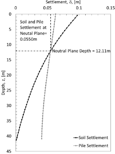
Table C9. Soil settlement and pile settlement as a function of depth.
| z | δp | δs | Comments: z=depth, Q=load, R=resistance, δp=pile settlement, δs=soil settlement, A=pile cross-sectional area=0.145[m2], Ep=pile elastic modulus=2.41E+07[kPa] Ls=length of each pile segment=0.8532[m] |
| [m] | [m] | [m] | |
| 0.4176 | 0.0635 | 0.0972 | |
| 1.2528 | 0.0630 | 0.0939 | |
| 2.088 | 0.0625 | 0.0905 | |
| 2.9232 | 0.0619 | 0.0872 | |
| 3.7584 | 0.0614 | 0.0839 | |
| 4.5936 | 0.0608 | 0.0806 | |
| 5.4288 | 0.0603 | 0.0774 | |
| 6.264 | 0.0598 | 0.0743 | |
| 7.0992 | 0.0592 | 0.0713 | |
| 7.9344 | 0.0586 | 0.0684 | |
| 8.7696 | 0.0581 | 0.0655 | |
| 9.6048 | 0.0575 | 0.0628 | |
| 10.44 | 0.0569 | 0.0601 | |
| 11.2752 | 0.0564 | 0.0575 | |
| 12.1104 | 0.0558 | 0.0550 | |
| 12.9456 | 0.0552 | 0.0526 | |
| 13.7808 | 0.0546 | 0.0503 | |
| 14.616 | 0.0540 | 0.0480 | |
| 15.4512 | 0.0534 | 0.0458 | |
| 16.2864 | 0.0528 | 0.0437 | |
| 17.1216 | 0.0522 | 0.0417 | |
| 17.9568 | 0.0516 | 0.0397 | |
| 18.792 | 0.0511 | 0.0378 | |
| 19.6272 | 0.0505 | 0.0359 | |
| 20.4624 | 0.0500 | 0.0341 | |
| 21.2976 | 0.0494 | 0.0323 | |
| 22.1328 | 0.0489 | 0.0306 | |
| 22.968 | 0.0484 | 0.0289 | |
| 23.8032 | 0.0479 | 0.0273 | |
| 24.6384 | 0.0474 | 0.0257 | |
| 25.4736 | 0.0469 | 0.0242 | |
| 26.3088 | 0.0464 | 0.0227 | |
| 27.144 | 0.0459 | 0.0213 | |
| 27.9792 | 0.0455 | 0.0198 | |
| 28.8144 | 0.0451 | 0.0185 | |
| 29.6496 | 0.0447 | 0.0171 | |
| 30.4848 | 0.0443 | 0.0158 | |
| 31.32 | 0.0439 | 0.0145 | |
| 32.1552 | 0.0435 | 0.0132 | |
| 32.9904 | 0.0432 | 0.0120 | |
| 33.8256 | 0.0429 | 0.0108 | |
| 34.6608 | 0.0426 | 0.0096 | |
| 35.496 | 0.0423 | 0.0085 | |
| 36.3312 | 0.0421 | 0.0073 | |
| 37.1664 | 0.0418 | 0.0062 | |
| 38.0016 | 0.0416 | 0.0051 | |
| 38.8368 | 0.0414 | 0.0041 | |
| 39.672 | 0.0413 | 0.0030 | |
| 40.5072 | 0.0412 | 0.0020 | |
| 41.3424 | 0.0411 | 0.0010 |

Conclusion:
Hand calculations were performed to determine the amount of drag load and downdrag on a pile being subjected to a change in effective stress from an embankment. Using the flowchart developed during the NCHRP 12-116A project, the downdrag, drag load, and location of the neutral plane were determined to be 0.055m, 286kN, and 13.36m, respectively. If the compressive strength of the concrete in the pile was 5000psi (34474kPa), the pile was determined to be adequately sized to support the loading conditions applied to the pile. This design approach relied upon the use of the DeCock (2009) method based on Chin’s Hyperbolic Model for determination of the load-settlement curve. Inherent assumptions in the design approach for determination of the load-settlement curve led to the suggestion that the neutral plane location determined using the combined load-resistance curve be used instead of the neutral plane location determined using the soil settlement-pile settlement curve.
References
Briaud, J.L., and Tucker, L. (1997). NCHRP Report 393: Design and Construction Guidelines for Downdrag on Uncoated and Bitumen-Coated Piles. TRB, National Research Council, Washington, DC.
Coffman, R.A., Budge, A.S., Stuedlein, A.W. (2022). “Report on Phase II Methodology and Design Procedures Interim Deliverable” NCHRP 12-116A Project Deliverable. Transportation Research Board. Version II, July 2022.
Davisson, M.T. (1972) “High Capacity Piles” Proceedings, Lecture Series, Innovations in Foundation Construction, ASCE, Illinois Section, 52 pp.
DeCock, F.A. (2009). Sense and Sensitivity of Pile Load-Deformation Behavior. Deep Foundation on Board and Auger Piles. Taylor and Francis. 22 pp.
Randolph, M.F., and Murphy, B.S. (1985). “Shaft Capacity of Driven Piles in Clay.” Proceedings of the 1985 Offshore Technology Conference. Paper No. OTC-4883-MS. May 6-9. Houston, TX.


